Half-life
From Wikipedia, the free encyclopedia
| Number of half-lives elapsed |
Fraction remaining |
Percentage remaining |
|
|---|---|---|---|
| 0 | 1/1 | 100 | |
| 1 | 1/2 | 50 | |
| 2 | 1/4 | 25 | |
| 3 | 1/8 | 12 | .5 |
| 4 | 1/16 | 6 | .25 |
| 5 | 1/32 | 3 | .125 |
| 6 | 1/64 | 1 | .563 |
| 7 | 1/128 | 0 | .781 |
| ... | ... | ... | |
| n | 1/2n | 100(1/2n) | |
The half-life of a quantity whose value decreases with time is the interval required for the quantity to decay to half of its initial value. The concept originated in describing how long it takes atoms to undergo radioactive decay but also applies in a wide variety of other situations.
The term "half-life" dates to 1907. The original term was "half-life period", but that was shortened to "half-life" starting in the early 1950s.[1]
Half-lives are very often used to describe quantities undergoing exponential decay—for example radioactive decay—where the half-life is constant over the whole life of the decay, and is a characteristic unit (a natural unit of scale) for the exponential decay equation. However, a half-life can also be defined for non-exponential decay processes, although in these cases the half-life varies throughout the decay process. For a general introduction and description of exponential decay, see the article exponential decay. For a general introduction and description of non-exponential decay, see the article rate law.
The converse for exponential growth is the doubling time.
The table at right shows the reduction of the quantity in terms of the number of half-lives elapsed.
Contents |
[edit] Probabilistic nature of half-life
A half-life often describes the decay of discrete entities, such as radioactive atoms. In that case, it does not work to use the definition "half-life is the time required for exactly half of the entities to decay". For example, if there is just one radioactive atom with a half-life of 1 second, there will not be "half of an atom" left after 1 second. There will be either zero atoms left or one atom left, depending on whether or not the atom happens to decay.
Instead, the half-life is defined in terms of probability. It is the time when the expected value of the number of entities that have decayed is equal to half the original number. For example, one can start with a single radioactive atom, wait its half-life, and measure whether or not it decays in that period of time. Perhaps it will and perhaps it will not. But if this experiment is repeated again and again, it will be seen that it decays within the half life 50% of the time.
In some experiments (such as the synthesis of a superheavy element), there is in fact only one radioactive atom produced at a time, with its lifetime individually measured. In this case, statistical analysis is required to infer the half-life. In other cases, a very large number of identical radioactive atoms decay in the time-range measured. In this case, the central limit theorem ensures that the number of atoms that actually decay is essentially equal to the number of atoms that are expected to decay. In other words, with a large enough number of decaying atoms, the probabilistic aspects of the process can be ignored.
There are various simple exercises that demonstrate probabilistic decay, for example involving flipping coins or running a computer program. See the following websites: [1], [2], [3].
[edit] Formulae for half-life in exponential decay
An exponential decay process can be described by any of the following three equivalent formulae:

- Nt = N0e − t / τ
- Nt = N0e − λt
where
-
- N0 is the initial quantity of the thing that will decay (this quantity may be measured in grams, moles, number of atoms, etc.),
- Nt is the quantity that still remains and has not yet decayed after a time t,
- t1 / 2 is the half-life of the decaying quantity,
- τ is a positive number called the mean lifetime of the decaying quantity,
- λ is a positive number called the decay constant of the decaying quantity.
The three parameters t1 / 2, τ, and λ are all directly related in the following way:
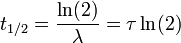
where ln(2) is the natural logarithm of 2 (approximately 0.693).
-
Click "show" to see a detailed derivation of the relationship between half-life, decay time, and decay constant. Start with the three equations - Nt = N0e − t / τ
- Nt = N0e − λt
We want to find a relationship between t1 / 2, τ, and λ, such that these three equations describe exactly the same exponential decay process. Comparing the equations, we find the following condition:
Next, we'll take the natural logarithm of each of these quantities.
Using the properties of logarithms, this simplifies to the following:
- (t / t1 / 2)ln(1 / 2) = ( − t / τ)ln(e) = ( − λt)ln(e)
Since the natural logarithm of e is 1, we get:
- (t / t1 / 2)ln(1 / 2) = − t / τ = − λt
Canceling the factor of t and plugging in ln(1 / 2) = − ln2, the eventual result is:


By plugging in and manipulating these relationships, we get all of the following equivalent descriptions of exponential decay, in terms of the half-life:


Regardless of how it's written, we can plug into the formula to get
- Nt = N0 at t=0 (as expected—this is the definition of "initial quantity")
- Nt = (1 / 2)N0 at t = t1 / 2 (as expected—this is the definition of half-life)
- Nt approaches zero when t approaches infinity (as expected—the longer we wait, the less remains).
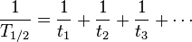
[edit] Decay by two or more processes
Some quantities decay by two exponential-decay processes simultaneously. In this case, the actual half-life T1/2 can be related to the half-lives t1 and t2 that the quantity would have if each of the decay processes acted in isolation:

For three or more processes, the analogous formula is:
For a proof of these formulae, see Decay by two or more processes.
[edit] Examples
There is a half-life describing any exponential-decay process. For example:
- The current flowing through an RC circuit or RL circuit decays with a half-life of RCln(2) or ln(2)L / R, respectively.
- In a first-order chemical reaction, the half-life of the reactant is ln(2) / λ, where λ is the reaction rate constant.
- In radioactive decay, the half-life is the length of time after which there is a 50% chance that an atom will have undergone nuclear decay. It varies depending on the atom type and isotope, and is usually determined experimentally.
[edit] Half-life in non-exponential decay
Many quantities decay in a way not described by exponential decay—for example, the evaporation of water from a puddle, or (often) the chemical reaction of a molecule. In this case, the half-life is defined the same way as before: The time elapsed before half of the original quantity has decayed. However, unlike in an exponential decay, the half-life depends on the initial quantity, and changes over time as the quantity decays.
As an example, the radioactive decay of carbon-14 is exponential with a half-life of 5730 years. If you have a quantity of carbon-14, half of it (on average) will have decayed after 5730 years, regardless of how big or small the original quantity was. If you wait another 5730 years, one-quarter of the original will remain. On the other hand, the time it will take a puddle to half-evaporate depends on how deep the puddle is. Perhaps a puddle of a certain size will evaporate down to half its original volume in one day. But if you wait a second day, there is no reason to expect that precisely one-quarter of the puddle will remain; in fact, it will probably be much less than that. This is an example where the half-life reduces as time goes on. (In other non-exponential decays, it can increase instead.)
For specific, quantitative examples of half-lives in non-exponential decays, see the article Rate equation.
A biological half-life is also a type of half-life associated with a non-exponential decay, namely the decay of the activity of a drug or other substance after it is introduced into the body.
[edit] See also
| Look up half-life in Wiktionary, the free dictionary. |
[edit] References
- ^ John Ayto, "20th Century Words" (1989), Cambridge University Press.

