Conditional probability

From Wikipedia, the free encyclopedia

Conditional probability is the probability of some event A, given the occurrence of some other event B. Conditional probability is written P(A|B), and is read "the probability of A, given B".

Joint probability is the probability of two events in conjunction. That is, it is the probability of both events together. The joint probability of A and B is written $\scriptstyle P(A \cap B)$ or $\scriptstyle P(A, B).$

Marginal probability is then the unconditional probability P(A) of the event A; that is, the probability of A, regardless of whether event B did or did not occur. If B can be thought of as the event of a random variable X having a given outcome, the marginal probability of A can be obtained by summing (or integrating, more generally) the joint probabilities over all outcomes for X. For example, if there are two possible outcomes for X with corresponding events B and B', this means that $\scriptstyle P(A) = P(A \cap B) + P(A \cap B^')$ . This is called marginalization.

In these definitions, note that there need not be a causal or temporal relation between A and B. A may precede B or vice versa or they may happen at the same time. A may cause B or vice versa or they may have no causal relation at all. Notice, however, that causal and temporal relations are informal notions, not belonging to the probabilistic framework. They may apply in some examples, depending on the interpretation given to events.

Conditioning of probabilities, i.e. updating them to take account of (possibly new) information, may be achieved through Bayes' theorem. In such conditioning, the probability of A given only initial information I, P(A|I), is known as the prior probability. The updated conditional probability of A, given I and the outcome of the event B, is known as the posterior probability, P(A|B,I).

[edit] Introduction

Consider the simple scenario of rolling two fair six-sided dice, labelled die 1 and die 2. Define the following three events:

A: Dice 1 lands on 3.

B: Dice 2 lands on 1.

C: The dice sum to 8.

The prior probability of each event describes how likely the outcome is before the dice are rolled, without any knowledge of the roll's outcome. For example, die 1 is equally likely to fall on each of its 6 sides, so P(A) = 1/6. Similarly P(B) = 1/6. Likewise, of the 6 × 6 = 36 possible ways that a pair of dice can land, just 5 result in a sum of 8 (namely 2 and 6, 3 and 5, 4 and 4, 5 and 3, and 6 and 2), so P(C) = 5/36.

Some of these events can both occur at the same time; for example events A and C can happen at the same time, in the case where die 1 lands on 3 and die 2 lands on 5. This is the only one of the 36 outcomes where both A and C occur, so its probability is 1/36. The probability of both A and C occurring is called the joint probability of A and C and is written $P(A \cap C)$ , so $P(A \cap C) = 1/36$ . On the other hand, if die 2 lands on 1, the dice cannot sum to 8, so $P(B \cap C) = 0$ .

Now suppose we roll the dice and cover up die 2, so we can only see die 1, and observe that die 1 landed on 3. Given this partial information, the probability that the dice sum to 8 is no longer 5/36; instead it is 1/6, since die 2 must land on 5 to achieve this result. This is called the conditional probability, because it is the probability of C under the condition that A is observed, and is written P(C | A), which is read "the probability of C given A." Similarly, P(C | B) = 0, since if we observe die 2 landed on 1, we already know the dice can't sum to 8, regardless of what the other die landed on.

On the other hand, if we roll the dice and cover up die 2, and observe die 1, this has no impact on the probability of event B, which only depends on die 2. We say events A and B are statistically independent or just independent and in this case

$P(B \mid A) = P(B) \, .$

In other words, the probability of B occurring after observing that die 1 landed on 3 is the same as before we observed die 1.

Intersection events and conditional events are related by the formula:

$P(C \mid A) = \frac{P(A \cap C)}{P(A)}.$

In this example, we have:

$1/6 = \frac{1/36}{1/6}$

As noted above, $P(B \mid A) = P(B)$ , so by this formula:

$P(B) = P(B \mid A) = \frac{P(A \cap B)}{P(A)} .$

On multiplying across by P(A),

$P(A)P(B) = P(A \cap B). \,$

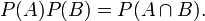
In other words, if two events are independent, their joint probability is the product of the prior probabilities of each event occurring by itself.

[edit] Definition

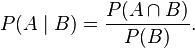
Given a probability space $\scriptstyle (\Omega, F, P)$ and two events $\scriptstyle A, B\,\in\, F$ with P(B) > 0, the conditional probability of A given B is defined by

$P(A \mid B) = \frac{P(A \cap B)}{P(B)}.\,$

If $P (B) = 0$ then $P(A \mid B)$ is undefined (see Borel–Kolmogorov paradox for an explanation). However it is possible to define a conditional probability with respect to a σ-algebra of such events (such as those arising from a continuous random variable). See conditional expectation for more information.

[edit] Derivation

The following derivation is taken from Grinstead and Snell's Introduction to Probability.^[1]

Let $\Omega = \{ \omega_1,\ldots,\omega_n \}$ be the original sample space, with elementary outcomes or elementary events $ω i$ , and the probability operation $P$ given as $P: \Omega \rightarrow [0,1]$ , for example $P(\omega_i) \in [0,1]$ .

Suppose event $E \subseteq \Omega$ has occurred and an altered probability $P (ω i | E)$ is to be assigned to the elementary events to reflect the fact that $E$ has occurred.

For all $\omega_j \not\in E$ we want to make sure that the intuitive result $P (ω j | E) = 0$ is true.

Also, without further information provided, we can be certain that the relative magnitude of probabilities is conserved:

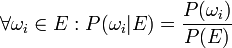
$\omega_i, \omega_k \in E: P(\omega_i) \leq P(\omega_k) \Rightarrow P(\omega_i | E) \leq P(\omega_k | E)$ .

This requirement leads us to state:

$\omega_i \in E: P(\omega_i | E) = \alpha \cdot P(\omega_i)$

where $\alpha \in \mathbb{R}^{+}$ , i.e. $α$ is a positive constant or scaling factor to reflect the above requirement.

Since we know $E$ has occurred, we can state

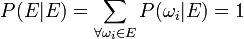
$P(E | E) = \sum_{\forall \omega_i \in E} {P(\omega_i | E)} = 1$

which allows us to say:

$\sum_{\forall \omega_i \in E} {P(\omega_i | E)} = \sum_{\forall \omega_i \in E} {\alpha \cdot P(\omega_i)} = \alpha \cdot \sum_{\forall \omega_i \in E} {P(\omega_i)} = 1$

From the above we obtain:

$\alpha = \frac{1}{\sum_{\forall \omega_i \in E} {P(\omega_i)}} = \frac{1}{P(E)} \iff P(E) > 0$

This leads us to state the following:

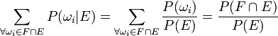
$\forall \omega_i \in E: P(\omega_i | E) = \frac{P(\omega_i)}{P(E)}$

Now for an event $F \subseteq \Omega$ and since $\forall \omega_j \not\in E: P(\omega_j | E) = 0$ :

$P(F|E) = \sum_{\forall \omega_k \in F} {P(\omega_k | E)} = \sum_{\forall \omega_i \in F \cap E} {P(\omega_i | E)} + \sum_{\forall \omega_j \not\in F \cap E} {\underbrace{P(\omega_j | E)}_{= 0}} =$

$\sum_{\forall \omega_i \in F \cap E} {P(\omega_i | E)} = \sum_{\forall \omega_i \in F \cap E} {\frac{P(\omega_i)}{P(E)}} = \frac{P(F \cap E)}{P(E)}$

[edit] Statistical independence

Two random events A and B are statistically independent if and only if

$P(A \cap B) \ = \ P(A) P(B)$

Thus, if A and B are independent, then their joint probability can be expressed as a simple product of their individual probabilities.

Equivalently, for two independent events A and B with non-zero probabilities,

$P(A|B) \ = \ P(A)$

and

$P(B|A) \ = \ P(B).$

In other words, if A and B are independent, then the conditional probability of A, given B is simply the individual probability of A alone; likewise, the probability of B given A is simply the probability of B alone.

[edit] Mutual exclusivity

Two events A and B are mutually exclusive if and only if $\scriptstyle A \cap B \,=\, \varnothing$ . Then $\scriptstyle P(A \cap B)\, =\, 0$ .

Therefore, if P(B) > 0 then $\scriptstyle P(A\mid B)$ is defined and equal to 0.

[edit] The conditional probability fallacy

Main article: Confusion of the inverse

The conditional probability fallacy is the assumption that P(A|B) is approximately equal to P(B|A). The mathematician John Allen Paulos discusses this in his book Innumeracy (p. 63 et seq.), where he points out that it is a mistake often made even by doctors, lawyers, and other highly educated non-statisticians. It can be overcome by describing the data in actual numbers rather than probabilities.

The relation between P(A|B) and P(B|A) is given by Bayes' theorem:

$P(B {\mid} A)= P(A {\mid} B) \, \frac{P(B)}{P(A)}.$

In other words, one can only assume that P(A|B) is approximately equal to P(B|A) if the prior probabilities P(A) and P(B) are also approximately equal.

[edit] An example

In the following constructed but realistic situation, the difference between P(A|B) and P(B|A) may be surprising, but is at the same time obvious.

In order to identify individuals having a serious disease in an early curable form, one may consider screening a large group of people. While the benefits are obvious, an argument against such screenings is the disturbance caused by false positive screening results: If a person not having the disease is incorrectly found to have it by the initial test, they will most likely be quite distressed until a more careful test shows that they do not have the disease. Even after being told they are well, their lives may be affected negatively.

The magnitude of this problem is best understood in terms of conditional probabilities.

Suppose 1% of the group suffer from the disease, and the rest are well. Choosing an individual at random,

P (ill) = 1% = 0.01 and P (well) = 99% = 0.99.

Suppose that when the screening test is applied to a person not having the disease, there is a 1% chance of getting a false positive result, i.e.

P (positive | well) = 1%, and P (negative | well) = 99%.

Finally, suppose that when the test is applied to a person having the disease, there is a 1% chance of a false negative result, i.e.

P (negative | ill) = 1% and P (positive | ill) = 99%.

Now, one may calculate the following:

The fraction of individuals in the whole group who are well and test negative:

$P(\text{well}\cap\text{negative})=P(\text{well})\times P(\text{negative}|\text{well})=99%\times99%=98.01%.$

The fraction of individuals in the whole group who are ill and test positive:

$P(\text{ill}\cap\text{positive}) = P(\text{ill})\times P(\text{positive}|\text{disease}) = 1%\times99% = 0.99%.$

The fraction of individuals in the whole group who have false positive results:

$P(\text{well}\cap\text{positive})=P(\text{well})\times P(\text{positive}|\text{well})=99%\times1%=0.99%.$

The fraction of individuals in the whole group who have false negative results:

$P(\text{ill}\cap\text{negative})=P(\text{ill})\times P(\text{negative}|\text{disease}) = 1%\times1% = 0.01%.$

Furthermore, the fraction of individuals in the whole group who test positive:

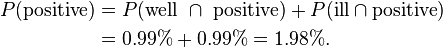
$\begin{align} P(\text{positive}) & {} =P(\text{well }\cap\text{ positive}) + P(\text{ill} \cap \text{positive}) \\ & {} = 0.99%+0.99%=1.98%. \end{align}$

Finally, the probability that an individual actually has the disease, given that the test result is positive:

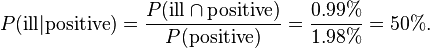
$P(\text{ill}|\text{positive})=\frac{P(\text{ill}\cap\text{positive})} {P(\text{positive})} = \frac{0.99%}{1.98%}= 50%.$

In this example, it should be easy to relate to the difference between the conditional probabilities P(positive | ill) (which is 99%) and P(ill | positive) (which is 50%): the first is the probability that an individual who has the disease tests positive; the second is the probability that an individual who tests positive actually has the disease. With the numbers chosen here, the last result is likely to be deemed unacceptable: half the people testing positive are actually false positives.

[edit] Second type of conditional probability fallacy

Another type of fallacy is interpreting conditional probabilities of events (or a series of events) as (unconditional) probabilities, or seeing them as being in the same order of magnitude. A conditional probability of an event and its (total) probability are linked with each other through the formula of total probability, but without additional information one of them says little about the other. The fallacy to view P(A|B) as P(A) or as being close to P(A) is often related with some forms of statistical bias but it can be subtle.

Here is an example: One of the conditions for the legendary wild-west hero Wyatt Earp to have become a legend was having survived all the duels he survived. Indeed, it is reported that he was never wounded, not even scratched by a bullet. The probability of this to happen is very small, contributing to his fame because events of very small probabilities attract attention. However, the point is that the degree of attention depends very much on the observer. Somebody impressed by a specific event (here seeing a "hero") is prone to view effects of randomness differently from others which are less impressed.

In general makes not much sense to ask after observation of a remarkable series of events "What is the probability of this?", because this is a conditional probability upon observation. The distinction between conditional and unconditional probabilities can be intricate if the observer who asks "What is the probability?" is himself/herself outcome of a random selection. The name "Wyatt Earp effect" was coined in an article "Der Wyatt Earp Effekt" (in German) showing through several examples its subtlety and impact in various scientific domains.

[edit] Conditioning on a random variable

There is also a concept of the conditional probability of an event given a discrete random variable. Such a conditional probability is a random variable in its own right.

Suppose X is a random variable that can be equal either to 0 or to 1. As above, one may speak of the conditional probability of any event A given the event X = 0, and also of the conditional probability of A given the event X = 1. The former is denoted P(A|X = 0) and the latter P(A|X = 1). Now define a new random variable Y, whose value is P(A|X = 0) if X = 0 and P(A|X = 1) if X = 1. That is

$Y = \begin{cases} P(A\mid X=0) & \text{if }X=0; \\ P(A\mid X=1) & \text{if }X=1. \end{cases}$

This new random variable Y is said to be the conditional probability of the event A given the discrete random variable X:

$Y = P(A\mid X). \,$

According to the "law of total probability", the expected value of Y is just the marginal (or "unconditional") probability of A.

More generally still, it is possible to speak of the conditional probability of an event given a sigma-algebra. See conditional expectation.

[edit] See also

[edit] References

^ Grinstead and Snell's Introduction to Probability, p. 142

Eric W. Weisstein, Conditional Probability at MathWorld.

F. Thomas Bruss Der Wyatt-Earp-Effekt oder die betoerende Macht kleiner Wahrscheinlichkeiten (in German), Spektrum der Wissenschaft (German Edition of Scientific American), Vol 2, 110–113, (2007).

[grinstead-0] Grinstead and Snell's Introduction to Probability, p. 142

[1]

Conditional probability

From Wikipedia, the free encyclopedia

Contents

[edit] Introduction

[edit] Definition

[edit] Derivation

[edit] Statistical independence

[edit] Mutual exclusivity

[edit] The conditional probability fallacy

[edit] An example

[edit] Second type of conditional probability fallacy

[edit] Conditioning on a random variable

[edit] See also

[edit] References

Views

Personal tools

Navigation

Search

Interaction

Toolbox

Languages