Effect size

From Wikipedia, the free encyclopedia

In statistics, effect size is a measure of the strength of the relationship between two variables. In scientific experiments, it is often useful to know not only whether an experiment has a statistically significant effect, but also the size of any observed effects. In practical situations, effect sizes are helpful for making decisions. Effect size measures are the common currency of meta-analysis studies that summarize the findings from a specific area of research.

[edit] Summary

The concept of effect size appears in everyday language. For example, a weight loss program may boast that it leads to an average weight loss of 30 pounds. In this case, 30 pounds is an indicator of the claimed effect size. Another example is that a tutoring program may claim that it raises school performance by one letter grade. This grade increase is the claimed effect size of the program.

An effect size is best explained through an example: if you had no previous contact with humans, and one day visited England, how many people would you need to see before you realize that, on average, men are taller than women there? The answer relates to the effect size of the difference in average height between men and women. The larger the effect size, the easier it is to see that men are taller. If the height difference were small, then it would require knowing the heights of many men and women to notice that (on average) men are taller than women. This example is demonstrated further below.

In inferential statistics, an effect size helps to determine whether a statistically significant difference is a difference of practical concern. In other words, given a sufficiently large sample size, it is always possible to show that there is a difference between two means being compared out to some decimal position. The effects size helps us to know whether the difference observed is a difference that matters. Effect size, sample size, critical significance level ( $α$ ), and power in statistical hypothesis testing are related: any one of these values can be determined, given the others. In meta-analysis, effect sizes are used as a common measure that can be calculated for different studies and then combined into overall analyses.

The term effect size more often refers to a statistic which relies on a replication of samples. However, just like the term variance, whether it means a population parameter or a samples' statistic, is contextual. In inferential statistics, the population parameter does not vary across replications or experiments, and has a confidence interval for each replication of samples, while the samples' statistic varies replication by replication, and usually converges to one corresponding population parameter as sample size increases infinitely. Conventionally, Greek letters like $ρ$ denote population parameters and Latin letters like r denote samples' statistics or point estimate. Currently, most named effect sizes have not made an explicit distinction. So, Cumming and Finch (2001) proposed using Cohen's $δ$ to denote the corresponding population parameter of Cohen's d. Another convention uses $\hat{\cdot}$ refer to sample or point estimate of some population symbol, and $\tilde{\cdot}$ to population of some sample or point estimate symbol. Following it, population of Cohen's $f 2$ is denoted $\tilde{f}^2$ and point estimate of $ω 2$ denoted $\hat{\omega}^2$ .

The term effect size is most commonly used to refer to standardized measures of effect (such as r, Cohen's d, and odds ratio). However, unstandardized measures (e.g., the raw difference between group means and unstandardized regression coefficients) can equally be effect size measures. Standardized effect size measures are typically used when the metrics of variables being studied do not have intrinsic meaning to the reader (e.g., a score on a personality test on an arbitrary scale), or when results from multiple studies are being combined when some or all of the studies use different scales. Some people mistook the recommendation of Wilkinson and APA Task Force on Statistical Inference (1999, p. 599)--Always present effect sizes for primary outcomes--as requiring standardized measures of effect like Cohen's d. But in the next sentence the authors added -- If the units of measurement are meaningful on a practical level (e.g., number of cigarettes smoked per day), then we usually prefer an unstandardized measure (regression coefficient or mean difference) to a standardized measure (r or d).

[edit] Recommendation

Presentation of effect size and confidence interval is highly recommended in biological journals ^[1]. Biologists should ultimately be interested in biological importance, which can be assessed using the magnitude of an effect, not statistical significance. Combined use of an effect size and its confidence interval enables someone to assess the relationship within data more effectively than the use of p values, regardless of statistical significance. Also, routine presentation of effect size will encourage researchers to view their results in the context of previous research and will facilitate incorporating results into future meta-analysis. However, issues surrounding publication bias towards statistically significant results, coupled with inadequate statistical power will lead to an overestimation of effect sizes, consequently affecting meta-analyses and power-analyses.^[2]

[edit] Types

[edit] Pearson r correlation

Pearson's r correlation, introduced by Karl Pearson, is one of the most widely used effect sizes. It can be used when the data are continuous or binary; thus the Pearson r is arguably the most versatile effect size. This was the first important effect size to be developed in statistics. Pearson's r can vary in magnitude from -1 to 1, with -1 indicating a perfect negative linear relation, 1 indicating a perfect positive linear relation, and 0 indicating no linear relation between two variables. Cohen (1988, 1992) gives the following guidelines for the social sciences: small effect size, r = 0.1; medium, r = 0.3; large, r = 0.5.

Another often-used measure of the strength of the relationship between two variables is the coefficient of determination (the square of r, referred to as "r-squared"). This is a measure of the proportion of variance shared by the two variables, and varies from 0 to 1. An r² of 0.21 means that 21% of the total variance is shared by the two variables.

[edit] Effect sizes based on means

A (population) effect size θ based on means usually considers the standardized mean difference between two populations^[3]^:78

$\theta = \frac{\mu_1 - \mu_2}{\sigma}$ ,

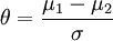where $μ 1$ is the mean for one population and $μ 2$ is the mean for the other population. σ is the standard deviation, — either of the second population or a standard deviation pooled from the two groups.

In the practical setting the population values are typically not known and must be estimated from sample statistics. The several versions of effect sizes based on means differ with respect to which statistics are used.

This form for the effect size resembles the computation for a t-test.

[edit] Cohen's d

Cohen's d is defined as the difference between two means divided by a standard deviation for the data

$d = \frac{\bar{x}_1 - \bar{x}_2}{s},$

What precisely the standard deviation s is was not originally made explicit by Jacob Cohen because he defined it (using the symbol "σ") as "the standard deviation of either population (since they are assumed equal)".^[4]^:20 Other authors make the computation of the standard deviation more explicit with the following definition for a pooled standard deviation^[5]^:14

$s = \sqrt{\frac{(n_1-1)s^2_1 + (n_2-1)s^2_2}{n_1+n_2} },$

with $\bar{x}_k$ and $s k$ as the mean and standard deviation for group k, for k = 1, 2.

$s_1^2 = \frac{1}{n_1-1} \sum_{i=1}^{n_1} (x_{1,i} - \bar{x}_1)^2$

This definition of "Cohen's d" is termed the maximum likelihood estimator by Hedges and Olkin, and it is related to Hedges' g (see below) by a scaling^[3]^:82

$g = \sqrt{\frac{n_1+n_2-2}{n_1+n_2}} d$

[edit] Glass's Δ

In 1976 Gene V. Glass proposed an estimator of the effect size that uses only the standard deviation of the second group^[3]^:78

$\Delta = \frac{\bar{x}_1 - \bar{x}_2}{s_2}$

The second group may be regarded as a control group, and Glass argued that if several treatments were compared to the control group it would be better to use just the standard deviation computed from the control group, so that effect sizes would not differ under equal means and different variances.

Under an assumption of equal population variances a pooled estimate for σ is more precise.

[edit] Hedges' g

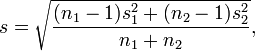
Hedges' g, suggested by Larry Hedges in 1981,^[6] is like the other measures based on a standardized difference^[3]^:79

$g = \frac{\bar{x}_1 - \bar{x}_2}{s^*}$

but its pooled standard deviation $s *$ is computed slightly differently from Cohen's d

$s^* = \sqrt{\frac{(n_1-1)s_1^2 + (n_2-1)s_2^2}{n_1+n_2-2}}$

As an estimator for the population effect size θ it is biased. However, this bias can be corrected for by multiplication with a factor

$g^* = J(n_1+n_2-2) g \approx \left(1-\frac{3}{4(n_1+n_2)-9}\right) g$

In their 1985 book Hedges and Olkin refer to this unbiased estimator $g *$ as d, but it is not the same as Cohen's d. The exact form for the correction factor J() involves the gamma function^[3]^:104

$J(a) = \frac{\Gamma(a/2)}{\sqrt{a/2}\Gamma((a-1)/2)}$

[edit] Distribution of effect sizes based on means

Provided that the data is Gaussian distributed a scaled Hedges' g, $\sqrt{(n_1 n_2/(n_1+n_2)}\,g$ , follows a noncentral t-distribution with the noncentrality parameter $\sqrt{(n_1 n_2/(n_1+n_2)}\theta$ and $n 1 + n 2 - 2$ degrees of freedom. Likewise, the scaled Glass' Δ is distributed with $n 2 - 1$ degrees of freedom.

From the distribution it is possible to compute the expectation and variance of the effect sizes.

In some cases large sample approximations for the variance are used. One suggestion for the variance of Hedges' unbiased estimator is^[3]^:86

$\hat{\sigma}^2(g^*) = \frac{n_1+n_2}{n_1 n_2} + \frac{(g^*)^2}{2(n_1 + n_2)}$

[edit] Cohen's $f 2$

Cohen's $f 2$ is an appropriate effect size measure to use in the context of an F-test for ANOVA or multiple regression. The $f 2$ effect size measure for multiple regression is defined as:

$f^{2} = {R^{2} \over 1 - R^{2}}$

where

R 2

is the squared multiple correlation.

The $f 2$ effect size measure for hierarchical multiple regression is defined as:

$f^{2} = {(R^{2}_{AB} - R^{2}_A) \over 1 - R^{2}_{AB}}$

where $R^{2}_A$ is the variance accounted for by a set of one or more independent variables A, and $R^{2}_{AB}$ is the combined variance accounted for by A and another set of one or more independent variables B.

By convention, $f 2$ effect sizes of 0.02, 0.15, and 0.35 are termed small, medium, and large, respectively (Cohen, 1988).

Cohen's $\hat{f}$ can also be found for factorial analysis of variance (ANOVA, aka the F-test) working backwards using :

$\hat{f}_{Effect} = {\sqrt{(df_{Effect}/N) (F_{Effect}-1)}}.$
In a balanced design (equivalent sample sizes across groups) of ANOVA, the corresponding population parameter of $f 2$ is : ${SS(\mu_1,\mu_2,\cdots,\mu_K)}\over{K \times \sigma^2}$ , wherein $μ j$ denotes the population mean within the j^th group of the total K groups, and $σ$ the equivalent population standard deviations within each groups. SS is the sum of squares manipulation in ANOVA.

[edit] φ, Cramér's φ, or Cramér's V

Phi (φ)	Cramér's Phi (φ_c)
$\phi = \sqrt{ \frac{\chi^2}{N}}$	$\phi_c = \sqrt{ \frac{\chi^2}{N(k - 1)}}$

The best measure of association for the chi-square test is phi (or Cramér's phi or V). Phi is related to the point-biserial correlation coefficient and Cohen's d and estimates the extent of the relationship between two variables (2 x 2).^[7] Cramér's Phi may be used with variables having more than two levels.

Phi can be computed by finding the square root of the chi-square statistic divided by the sample size.

Similarly, Cramér's phi is computed by taking the square root of the chi-square statistic divided by the sample size and the length of the minimum dimension (k is the smaller of the number of rows r or columns c).

φ_c is the intercorrelation of the two discrete variables^[8] and may be computed for any value of r or c. However, as chi-square values tend to increase with the number of cells, the greater the difference between r and c, the more likely φ_c will tend to 1 without strong evidence of a meaningful correlation.

Cramér's phi may also be applied to 'goodness of fit' chi-square models (i.e. those where c=1). In this case it functions as a measure of tendency towards a single outcome (i.e. out of k outcomes).

[edit] Odds ratio

The odds ratio is another useful effect size. It is appropriate when both variables are binary. For example, consider a study on spelling. In a control group, two students pass the class for every one who fails, so the odds of passing are two to one (or more briefly 2/1 = 2). In the treatment group, six students pass for every one who fails, so the odds of passing are six to one (or 6/1 = 6). The effect size can be computed by noting that the odds of passing in the treatment group are three times higher than in the control group (because 6 divided by 2 is 3). Therefore, the odds ratio is 3. However, odds ratio statistics are on a different scale to Cohen's d. So, this '3' is not comparable to a Cohen's d of '3'.

[edit] Confidence interval and relation to noncentral parameters

Confidence interval of unstandardized effect size like difference of means $(μ 1 - μ 2)$ can be found in common statistics textbooks and software, while confidence intervals of standardized effect size, especially Cohen's $\tilde{d}:=\frac{\mu_1-\mu_2}{\sigma}$ and $\tilde{f}^2:=\frac{SS(\mu_1,\mu_2,...,\mu_K)}{K \cdot \sigma^2}$ , rely on the calculation of confidence intervals of noncentral parameters (ncp). A common approach to construct $(1 - α)$ confidence interval of ncp is to find the critical ncp values to fit the observed statistic to tail quantiles $α / 2$ and $(1 - α / 2)$ . SAS and R-package MBESS provide functions for critical ncp. An online calculator based on R and MediaWiki provides interactive interface, which requires no coding and welcomes copy-left collaboration.

[edit] T test for mean difference of single group or two related groups

In case of single group, M ( $μ$ ) denotes the sample (population) mean of single group , and SD ( $σ$ ) denotes the sample (population) standard deviation. N is the sample size of the group. T test is used for the hypothesis on the difference between mean and a baseline $μ b a s e l i n e$ . Usually, $μ b a s e l i n e$ is zero, while not necessary. In case of two related groups, the single group is constructed by difference in each pair of samples, while SD ( $σ$ ) denotes the sample (population) standard deviation of differences rather than within original two groups.

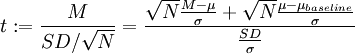
$t:=\frac{M}{SD/\sqrt{N}}=\frac{\sqrt{N}\frac{M-\mu}{\sigma} + \sqrt{N}\frac{\mu-\mu_{baseline}}{\sigma}}{\frac{SD}{\sigma}}$

$ncp=\sqrt{N}\frac{\mu-\mu_{baseline}}{\sigma}$ and Cohen's $d:=\frac{M-\mu_{baseline}}{SD}$ is the point estimate of $\frac{\mu-\mu_{baseline}}{\sigma}$ .

So,

$\tilde{d}=\frac{ncp}{\sqrt{N}}$ .

[edit] T test for mean difference between two independent groups

$n 1$ or $n 2$ is sample size within the respective group.

$t:=\frac{M_1-M_2}{SD_{within}/\sqrt{\frac{n_1 n_2}{n_1+n_2}}}$ , wherein $SD_{within}:=\sqrt{\frac{SS_{within}}{df_{within}}}=\sqrt{\frac{(n_1-1)SD_1^2+(n_2-1)SD_2^2}{n_1+n_2-2}}$ .

$ncp=\sqrt{\frac{n_1 n_2}{n_1+n_2}}\frac{\mu_1-\mu_2}{\sigma}$ and Cohen's $d:=\frac{M_1-M_2}{SD_{within}}$ is the point estimate of $\frac{\mu_1-\mu_2}{\sigma}$ .

So,

$\tilde{d}=\frac{ncp}{\sqrt{\frac{n_1 n_2}{n_1+n_2}}}$ .

[edit] One-way ANOVA test for mean difference across multiple independent groups

One-way ANOVA test applies noncentral F distribution. While with a given population standard deviation $σ$ , the same test question applies noncentral chi-square distribution.

$F:=\frac{\frac{SS_{between}}{\sigma^{2}}/df_{between}}{\frac{SS_{within}}{\sigma^{2}}/df_{within}}$

For each j-th sample within i-th group $X i, j$ , denote 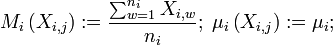$M_{i}\left(X_{i,j}\right):=\frac{\sum_{w=1}^{n_{i}}X_{i,w}}{n_{i}};\;\mu_{i}\left(X_{i,j}\right):=\mu_{i};$ .

While,

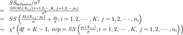$\begin{array}{ll} & SS_{between}/\sigma^{2}\\ = & \frac{SS\left(M_{i}\left(X_{i,j}\right);i=1,2,\cdots,K,\; j=1,2,\cdots,n_{i}\right)}{\sigma^{2}}\\ = & SS\left(\frac{M_{i}\left(X_{i,j}-\mu_{i}\right)}{\sigma}+\frac{\mu_{i}}{\sigma};i=1,2,\cdots,K,\; j=1,2,\cdots,n_{i}\right)\\ \sim & \chi^{2}\left(df=K-1,\; ncp=SS\left(\frac{\mu_i\left(X_{i,j}\right)}{\sigma};i=1,2,\cdots,K,\; j=1,2,\cdots,n_{i}\right)\right)\end{array}$ .

So, both ncp(s) of F and $χ 2$ equate

$SS\left(\mu_i(X_{i,j})/\sigma;i=1,2,\cdots,K,\; j=1,2,\cdots,n_{i}\right)$ .

In case of $n:=n_1=n_2=\cdots=n_K$ for K independent groups of same size, the total sample size is $N:=n\cdot K$ .

$Cohen's\;\tilde{f}{}^{2}:=\frac{SS(\mu_{1},\mu_{2},...,\mu_{K})}{K\cdot\sigma^{2}}=\frac{SS\left(\mu_i\left(X_{i,j}\right)/\sigma;i=1,2,\cdots,K,\; j=1,2,\cdots,n_{i}\right)}{n\cdot K}=\frac{ncp}{n\cdot K}=\frac{ncp}N$ .

T-test of pair of independent groups is a special case of one-way ANOVA. Note that noncentral parameter $n c p F$ of F is not comparable to the noncentral parameter $n c p t$ of the corresponding t. Actually, $ncp_F=ncp_t^2$ , and $\tilde{f}=\left|\frac{\tilde{d}}{2}\right|$ in the case.

[edit] "Small", "medium", "large"

Some fields using effect sizes apply words such as "small", "medium" and "large" to the size of the effect. Whether an effect size should be interpreted small, medium, or big depends on its substantial context and its operational definition. Cohen's (1988) conventional criterions small, medium, or big are near ubiquitous across many fields. Power analysis or sample size planning requires an assumed population parameter of effect sizes. Many researchers adopt Cohen's standards as default alternative hypotheses. Russell Lenth criticized them as T-shirt effect sizes^[9]

This is an elaborate way to arrive at the same sample size that has been used in past social science studies of large, medium, and small size (respectively). The method uses a standardized effect size as the goal. Think about it: for a "medium" effect size, you'll choose the same n regardless of the accuracy or reliability of your instrument, or the narrowness or diversity of your subjects. Clearly, important considerations are being ignored here. "Medium" is definitely not the message!

For Cohen's d an effect size of 0.2 to 0.3 might be a "small" effect, around 0.5 a "medium" effect and 0.8 to infinity, a "large" effect.^[4]^:25 (But note that the d might be larger than one)

In fact, in Cohen's (1988) text, he anticipates Lenth's concerns:

"The terms 'small,' 'medium,' and 'large' are relative, not only to each other, but to the area of behavioral science or even more particularly to the specific content and research method being employed in any given investigation....In the face of this relativity, there is a certain risk inherent in offering conventional operational definitions for these terms for use in power analysis in as diverse a field of inquiry as behavioral science. This risk is nevertheless accepted in the belief that more is to be gained than lost by supplying a common conventional frame of reference which is recommended for use only when no better basis for estimating the ES index is available." (p. 25)

The last two decades have seen the widespread use of these conventional (t-shirt) operational definitions as standard practice in the calculation of sample sizes despite the fact that Cohen was clear that the small-medium-large categories were not to be used by serious researchers, except perhaps in the context of research with entirely novel variables.

[edit] References

^ Nakagawa, S & Cuthill, IC. (2007) Effect size, confidence interval and statistical significance: a practical guide for biologists. Biological Reviews, 82, 591 - 605.
^ Brand A, Bradley MT, Best LA, Stoica G (April 2008). "Accuracy of effect size estimates from published psychological research". Perceptual and Motor Skills 106 (2): 645–649. http://mtbradley.com/brandbradelybeststoicapdf.pdf.
^ ^a ^b ^c ^d ^e ^f Larry V. Hedges & Ingram Olkin (1985). Statistical Methods for Meta-Analysis. Orlando: Academic Press. ISBN 0-12-336380-2.
^ ^a ^b Jacob Cohen (1988). Statistical Power Analysis for the Behavioral Sciences (second ed.). Lawrence Erlbaum Associates.
^ Joachim Hartung, Guido Knapp & Bimal K. Sinha (2008). Statistical Meta-Analysis with Application. Hoboken, New Jersey: Wiley.
^ Larry V. Hedges (1981). "Distribution theory for Glass's estimator of effect size and related estimators". Journal of Educational Statistics 6 (2): 107–128. doi:10.3102/10769986006002107.
^ Aaron, B., Kromrey, J. D., & Ferron, J. M. (1998, November). Equating r-based and d-based effect-size indices: Problems with a commonly recommended formula. Paper presented at the annual meeting of the Florida Educational Research Association, Orlando, FL. (ERIC Document Reproduction Service No. ED433353)
^ Sheskin, David J. (1997). Handbook of Parametric and Nonparametric Statistical Procedures. Boca Raton, Fl: CRC Press.
^ Russell V. Lenth. "Java applets for power and sample size". Division of Mathematical Sciences, the College of Liberal Arts or The University of Iowa. http://www.stat.uiowa.edu/~rlenth/Power/. Retrieved on 2008-10-08.

[edit] Further reading

Aaron, B., Kromrey, J. D., & Ferron, J. M. (1998, November). Equating r-based and d-based effect-size indices: Problems with a commonly recommended formula. Paper presented at the annual meeting of the Florida Educational Research Association, Orlando, FL. (ERIC Document Reproduction Service No. ED433353)
Cohen, J. (1992). A power primer. Psychological Bulletin, 112, 155-159.
Cumming, G. and Finch, S. (2001). A primer on the understanding, use, and calculation of confidence intervals that are based on central and noncentral distributions. Educational and Psychological Measurement, 61, 530–572.
Lipsey, M.W., & Wilson, D.B. (2001). Practical meta-analysis. Sage: Thousand Oaks, CA.
Wilkinson, L., & APA Task Force on Statistical Inference. (1999). Statistical methods in psychology journals: Guidelines and explanations. American Psychologist, 54, 594-604.

[edit] External links

Wikiversity has learning materials about Effect size

Software

Free Effect Size Generator - PC & Mac Software
MBESS - One of R's packages providing confidence intervals of effect sizes based non-central parameters
Free GPower Software - PC & Mac Software
Free Effect Size Calculator for Multiple Regression - Web Based
Free Effect Size Calculator for Hierarchical Multiple Regression - Web Based
Copylefted Online Calculator for Noncentral t, Chisquare, and F Distributions - Collaborated Wiki Page Powered by R
ES-Calc: a free add-on for Effect Size Calculation in ViSta 'The Visual Statistics System'. Computes Cohen's d, Glass's Delta, Hedges' g, CLES, Non-Parametric Cliff’s Delta, d-to-r Conversion, etc.

Further Explanations

[0] Nakagawa, S & Cuthill, IC. (2007) Effect size, confidence interval and statistical significance: a practical guide for biologists. Biological Reviews, 82, 591 - 605.

[1] Brand A, Bradley MT, Best LA, Stoica G (April 2008). "Accuracy of effect size estimates from published psychological research". Perceptual and Motor Skills 106 (2): 645–649. http://mtbradley.com/brandbradelybeststoicapdf.pdf.

[HedgesL1985Statistical-2] ^ ^a ^b ^c ^d ^e ^f Larry V. Hedges & Ingram Olkin (1985). Statistical Methods for Meta-Analysis. Orlando: Academic Press. ISBN 0-12-336380-2.

[CohenJ1988Statistical-3] Jacob Cohen (1988). Statistical Power Analysis for the Behavioral Sciences (second ed.). Lawrence Erlbaum Associates.

[4] Joachim Hartung, Guido Knapp & Bimal K. Sinha (2008). Statistical Meta-Analysis with Application. Hoboken, New Jersey: Wiley.

[5] Larry V. Hedges (1981). "Distribution theory for Glass's estimator of effect size and related estimators". Journal of Educational Statistics 6 (2): 107–128. doi:10.3102/10769986006002107.

[6] Aaron, B., Kromrey, J. D., & Ferron, J. M. (1998, November). Equating r-based and d-based effect-size indices: Problems with a commonly recommended formula. Paper presented at the annual meeting of the Florida Educational Research Association, Orlando, FL. (ERIC Document Reproduction Service No. ED433353)

[7] Sheskin, David J. (1997). Handbook of Parametric and Nonparametric Statistical Procedures. Boca Raton, Fl: CRC Press.

[8] Russell V. Lenth. "Java applets for power and sample size". Division of Mathematical Sciences, the College of Liberal Arts or The University of Iowa. http://www.stat.uiowa.edu/~rlenth/Power/. Retrieved on 2008-10-08.

[1]

[2]

[3]

[4]

[5]

[6]

[7]

[8]

[9]

Effect size

From Wikipedia, the free encyclopedia

Contents

[edit] Summary

[edit] Recommendation

[edit] Types

[edit] Pearson r correlation

[edit] Effect sizes based on means

[edit] Cohen's d

[edit] Glass's Δ

[edit] Hedges' g

[edit] Distribution of effect sizes based on means

[edit] Cohen's $f 2$

[edit] φ, Cramér's φ, or Cramér's V

[edit] Odds ratio

[edit] Confidence interval and relation to noncentral parameters

[edit] T test for mean difference of single group or two related groups

[edit] T test for mean difference between two independent groups

[edit] One-way ANOVA test for mean difference across multiple independent groups

[edit] "Small", "medium", "large"

[edit] References

[edit] Further reading

[edit] External links

Views

Personal tools

Navigation

Search

Interaction

Toolbox

Languages

Effect size

From Wikipedia, the free encyclopedia

Contents

[edit] Summary

[edit] Recommendation

[edit] Types

[edit] Pearson r correlation

[edit] Effect sizes based on means

[edit] Cohen's d

[edit] Glass's Δ

[edit] Hedges' g

[edit] Distribution of effect sizes based on means

[edit] Cohen's f2

[edit] φ, Cramér's φ, or Cramér's V

[edit] Odds ratio

[edit] Confidence interval and relation to noncentral parameters

[edit] T test for mean difference of single group or two related groups

[edit] T test for mean difference between two independent groups

[edit] One-way ANOVA test for mean difference across multiple independent groups

[edit] "Small", "medium", "large"

[edit] References

[edit] Further reading

[edit] External links

Views

Personal tools

Navigation

Search

Interaction

Toolbox

Languages

[edit] Cohen's $f 2$