Perceptron
From Wikipedia, the free encyclopedia
The perceptron is a type of artificial neural network invented in 1957 at the Cornell Aeronautical Laboratory by Frank Rosenblatt. It can be seen as the simplest kind of feedforward neural network: a linear classifier.
Contents |
[edit] Definition
The Perceptron uses matrix eigenvalues to represent feedforward neural networks and is a binary classifier that maps its input x (a real-valued vector) to an output value f(x) (a single binary value) across the matrix.
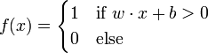
where w is a vector of real-valued weights and  is the dot product (which computes a weighted sum). b is the 'bias', a constant term that does not depend on any input value.
The value of f(x) (0 or 1) is used to classify x as either a positive or a negative instance, in the case of a binary classification problem. The bias can be thought of as offsetting the activation function, or giving the output neuron a "base" level of activity. If b is negative, then the weighted combination of inputs must produce a positive value greater than − b in order to push the classifier neuron over the 0 threshold. Spatially, the bias alters the position (though not the orientation) of the decision boundary.
Since the inputs are fed directly to the output unit via the weighted connections, the perceptron can be considered the simplest kind of feed-forward neural network.
[edit] Learning algorithm
The learning algorithm is the same across all neurons, therefore everything that follows is applied to a single neuron in isolation. We first define some variables:
- x(j) denotes the j-th item in the n-dimensional input vector
- w(j) denotes the j-th item in the weight vector
- f(x) denotes the output from the neuron when presented with input x
- α is a constant where
 (learning rate)
Further, assume for convenience that the bias term b is zero. This is not a restriction since an extra dimension n + 1 can be added to the input vectors x with x(n + 1) = 1, in which case w(n + 1) replaces the bias term.

Learning is modeled as the weight vector being updated for multiple iterations over all training examples. Let  denote a training set of m training examples.
Each iteration the weight vector is updated as follows:
For each (x,y) pair in

Note that this means that a change in the weight vector will only take place for a given training example (x,y) if its output f(x) is different from the desired output y.
The initialization of w is usually performed simply by setting w(j): = 0 for all elements w(j).
The training set Dm is said to be linearly separable if there exists a positive constant γ and a weight vector w such that  for all i. Novikoff (1962) proved that the perceptron algorithm converges after a finite number of iterations if the data set is linearly separable and the number of mistakes is bounded by
  where R the maximum norm of an input vector.
However, if the training set is not linearly separable, the above online algorithm is not guaranteed to converge.
Note that the decision boundary of a perceptron is invariant with respect to scaling of the weight vector, i.e. a perceptron trained with initial weight vector w and learning rate α is an identical estimator to a perceptron trained with initial weight vector w / α and learning rate 1. Thus, since the initial weights become irrelevant with increasing number of iterations, the learning rate does not matter in the case of the perceptron and is usually just set to one.
[edit] Variants
The pocket algorithm with ratchet (Gallant, 1990) solves the stability problem of perceptron learning by keeping the best solution seen so far "in its pocket". The pocket algorithm then returns the solution in the pocket, rather than the last solution.
The α-perceptron further utilised a preprocessing layer of fixed random weights, with thresholded output units. This enabled the perceptron to classify analogue patterns, by projecting them into a binary space. In fact, for a projection space of sufficiently high dimension, patterns can become linearly separable.
As an example, consider the case of having to classify data into two classes. Here is a small such data set, consisting of two points coming from two Gaussian distributions.
 Two class gaussian data |
 A linear classifier operating on the original space |
 A linear classifier operating on a high-dimensional projection |
A linear classifier can only separate things with a hyperplane, so it's not possible to classify all the examples perfectly. On the other hand, we may project the data into a large number of dimensions. In this case a random matrix was used to project the data linearly to a 1000-dimensional space; then each resulting data point was transformed through the hyperbolic tangent function. A linear classifier can then separate the data, as shown in the third figure. However the data may still not be completely separable in this space, in which the perceptron algorithm would not converge. In the example shown, stochastic steepest gradient descent was used to adapt the parameters.
Furthermore, by adding nonlinear layers between the input and output, one can separate all data and indeed, with enough training data, model any well-defined function to arbitrary precision. This model is a generalization known as a multilayer perceptron.
It should be kept in mind, however, that the best classifier is not necessarily that which classifies all the training data perfectly. Indeed, if we had the prior constraint that the data come from equi-variant Gaussian distributions, the linear separation in the input space is optimal.
Other training algorithms for linear classifiers are possible: see, e.g., support vector machine and logistic regression.
[edit] Example
A perceptron (X1, X2 input, X0*W0=b, TH=0.5) learns how to perform a NAND function:
| Input | Initial | Output | Final | |||||||||||||||
| Threshold | Learning Rate | Sensor values | Desired output | Weights | Calculated | Sum | Network | Error | Correction | Weights | ||||||||
| TH | LR | X0 | X1 | X2 | Z | w0 | w1 | w2 | C0 | C1 | C2 | S | N | E | R | W0 | W1 | W2 |
| X0 x w0 | X1 x w1 | X2 x w2 | C0+C1+C2 | IF(S>TH,1,0) | Z-N | LR x E | ||||||||||||
| 0.5 | 0.1 | 1 | 0 | 0 | 1 | 0 | 0 | 0 | 0 | 0 | 0 | 0 | 0 | 1 | +0.1 | 0.1 | 0 | 0 |
| 0.5 | 0.1 | 1 | 0 | 1 | 1 | 0.1 | 0 | 0 | 0.1 | 0 | 0 | 0.1 | 0 | 1 | +0.1 | 0.2 | 0 | 0.1 |
| 0.5 | 0.1 | 1 | 1 | 0 | 1 | 0.2 | 0 | 0.1 | 0.2 | 0 | 0 | 0.2 | 0 | 1 | +0.1 | 0.3 | 0.1 | 0.1 |
| 0.5 | 0.1 | 1 | 1 | 1 | 0 | 0.3 | 0.1 | 0.1 | 0.3 | 0.1 | 0.1 | 0.5 | 0 | 0 | 0 | 0.3 | 0.1 | 0.1 |
| 0.5 | 0.1 | 1 | 0 | 0 | 1 | 0.3 | 0.1 | 0.1 | 0.3 | 0 | 0 | 0.3 | 0 | 1 | +0.1 | 0.4 | 0.1 | 0.1 |
| 0.5 | 0.1 | 1 | 0 | 1 | 1 | 0.4 | 0.1 | 0.1 | 0.4 | 0 | 0.1 | 0.5 | 0 | 1 | +0.1 | 0.5 | 0.1 | 0.2 |
| 0.5 | 0.1 | 1 | 1 | 0 | 1 | 0.5 | 0.1 | 0.2 | 0.5 | 0.1 | 0 | 0.6 | 1 | 0 | 0 | 0.5 | 0.1 | 0.2 |
| 0.5 | 0.1 | 1 | 1 | 1 | 0 | 0.5 | 0.1 | 0.2 | 0.5 | 0.1 | 0.2 | 0.8 | 1 | -1 | -0.1 | 0.4 | 0 | 0.1 |
| 0.5 | 0.1 | 1 | 0 | 0 | 1 | 0.4 | 0 | 0.1 | 0.4 | 0 | 0 | 0.4 | 0 | 1 | +0.1 | 0.5 | 0 | 0.1 |
| 0.5 | 0.1 | 1 | 0 | 1 | 1 | 0.5 | 0 | 0.1 | 0.5 | 0 | 0.1 | 0.6 | 1 | 0 | 0 | 0.5 | 0 | 0.1 |
| 0.5 | 0.1 | 1 | 1 | 0 | 1 | 0.5 | 0 | 0.1 | 0.5 | 0 | 0 | 0.5 | 0 | 1 | +0.1 | 0.6 | 0.1 | 0.1 |
| 0.5 | 0.1 | 1 | 1 | 1 | 0 | 0.6 | 0.1 | 0.1 | 0.6 | 0.1 | 0.1 | 0.8 | 1 | -1 | -0.1 | 0.5 | 0 | 0 |
| 0.5 | 0.1 | 1 | 0 | 0 | 1 | 0.5 | 0 | 0 | 0.5 | 0 | 0 | 0.5 | 0 | 1 | +0.1 | 0.6 | 0 | 0 |
| 0.5 | 0.1 | 1 | 0 | 1 | 1 | 0.6 | 0 | 0 | 0.6 | 0 | 0 | 0.6 | 1 | 0 | 0 | 0.6 | 0 | 0 |
| 0.5 | 0.1 | 1 | 1 | 0 | 1 | 0.6 | 0 | 0 | 0.6 | 0 | 0 | 0.6 | 1 | 0 | 0 | 0.6 | 0 | 0 |
| 0.5 | 0.1 | 1 | 1 | 1 | 0 | 0.6 | 0 | 0 | 0.6 | 0 | 0 | 0.6 | 1 | -1 | -0.1 | 0.5 | -0.1 | -0.1 |
| 0.5 | 0.1 | 1 | 0 | 0 | 1 | 0.5 | -0.1 | -0.1 | 0.5 | 0 | 0 | 0.5 | 0 | 1 | +0.1 | 0.6 | -0.1 | -0.1 |
| 0.5 | 0.1 | 1 | 0 | 1 | 1 | 0.6 | -0.1 | -0.1 | 0.6 | 0 | -0.1 | 0.5 | 0 | 1 | +0.1 | 0.7 | -0.1 | 0 |
| 0.5 | 0.1 | 1 | 1 | 0 | 1 | 0.7 | -0.1 | 0 | 0.7 | -0.1 | 0 | 0.6 | 1 | 0 | 0 | 0.7 | -0.1 | 0 |
| 0.5 | 0.1 | 1 | 1 | 1 | 0 | 0.7 | -0.1 | 0 | 0.7 | -0.1 | 0 | 0.6 | 1 | -1 | -0.1 | 0.6 | -0.2 | -0.1 |
| 0.5 | 0.1 | 1 | 0 | 0 | 1 | 0.6 | -0.2 | -0.1 | 0.6 | 0 | 0 | 0.6 | 1 | 0 | 0 | 0.6 | -0.2 | -0.1 |
| 0.5 | 0.1 | 1 | 0 | 1 | 1 | 0.6 | -0.2 | -0.1 | 0.6 | 0 | -0.1 | 0.5 | 0 | 1 | +0.1 | 0.7 | -0.2 | 0 |
| 0.5 | 0.1 | 1 | 1 | 0 | 1 | 0.7 | -0.2 | 0 | 0.7 | -0.2 | 0 | 0.5 | 0 | 1 | +0.1 | 0.8 | -0.1 | 0 |
| 0.5 | 0.1 | 1 | 1 | 1 | 0 | 0.8 | -0.1 | 0 | 0.8 | -0.1 | 0 | 0.7 | 1 | -1 | -0.1 | 0.7 | -0.2 | -0.1 |
| 0.5 | 0.1 | 1 | 0 | 0 | 1 | 0.7 | -0.2 | -0.1 | 0.7 | 0 | 0 | 0.7 | 1 | 0 | 0 | 0.7 | -0.2 | -0.1 |
| 0.5 | 0.1 | 1 | 0 | 1 | 1 | 0.7 | -0.2 | -0.1 | 0.7 | 0 | -0.1 | 0.6 | 1 | 0 | 0 | 0.7 | -0.2 | -0.1 |
| 0.5 | 0.1 | 1 | 1 | 0 | 1 | 0.7 | -0.2 | -0.1 | 0.7 | -0.2 | 0 | 0.5 | 0 | 1 | +0.1 | 0.8 | -0.1 | -0.1 |
| 0.5 | 0.1 | 1 | 1 | 1 | 0 | 0.8 | -0.1 | -0.1 | 0.8 | -0.1 | -0.1 | 0.6 | 1 | -1 | -0.1 | 0.7 | -0.2 | -0.2 |
| 0.5 | 0.1 | 1 | 0 | 0 | 1 | 0.7 | -0.2 | -0.2 | 0.7 | 0 | 0 | 0.7 | 1 | 0 | 0 | 0.7 | -0.2 | -0.2 |
| 0.5 | 0.1 | 1 | 0 | 1 | 1 | 0.7 | -0.2 | -0.2 | 0.7 | 0 | -0.2 | 0.5 | 0 | 1 | +0.1 | 0.8 | -0.2 | -0.1 |
| 0.5 | 0.1 | 1 | 1 | 0 | 1 | 0.8 | -0.2 | -0.1 | 0.8 | -0.2 | 0 | 0.6 | 1 | 0 | 0 | 0.8 | -0.2 | -0.1 |
| 0.5 | 0.1 | 1 | 1 | 1 | 0 | 0.8 | -0.2 | -0.1 | 0.8 | -0.2 | -0.1 | 0.5 | 0 | 0 | 0 | 0.8 | -0.2 | -0.1 |
| 0.5 | 0.1 | 1 | 0 | 0 | 1 | 0.8 | -0.2 | -0.1 | 0.8 | 0 | 0 | 0.8 | 1 | 0 | 0 | 0.8 | -0.2 | -0.1 |
| 0.5 | 0.1 | 1 | 0 | 1 | 1 | 0.8 | -0.2 | -0.1 | 0.8 | 0 | -0.1 | 0.7 | 1 | 0 | 0 | 0.8 | -0.2 | -0.1 |
Note: Initial weight equals final weight of previous iteration. A too high learning rate makes the perceptron periodically oscillate around the solution. A possible enhancement is to use LRn starting with n=1 and incrementing it by 1 when a loop in learning is found.
[edit] Multiclass perceptron
Like most other techniques for training linear classifiers, the perceptron generalizes naturally to multiclass classification. Here, the input x and the output y are drawn from arbitrary sets. A feature representation function f(x,y) maps each possible input/output pair to a finite-dimensional real-valued feature vector. As before, the feature vector is multiplied by a weight vector w, but now the resulting score is used to choose among many possible outputs:
Learning again iterates over the examples, predicting an output for each, leaving the weights unchanged when the predicted output matches the target, and changing them when it does not. The update becomes:

This multiclass formulation reduces to the original perceptron when x is a real-valued vector, y is chosen from {0,1}, and f(x,y) = yx.
For certain problems, input/output representations and features can be chosen so that  can be found efficiently even though y is chosen from a very large or even infinite set.
In recent years, perceptron training has become popular in the field of natural language processing for such tasks as part-of-speech tagging and syntactic parsing (Collins, 2002).
[edit] History
- See also: History of artificial intelligence, AI Winter and Frank Rosenblatt
Although the perceptron initially seemed promising, it was eventually proved that perceptrons could not be trained to recognise many classes of patterns. This led to the field of neural network research stagnating for many years, before it was recognised that a feedforward neural network with two or more layers (also called a multilayer perceptron) had far greater processing power than perceptrons with one layer (also called a single layer perceptron). Single layer perceptrons are only capable of learning linearly separable patterns; in 1969 a famous book entitled Perceptrons by Marvin Minsky and Seymour Papert showed that it was impossible for these classes of network to learn an XOR function. They conjectured (incorrectly) that a similar result would hold for a perceptron with three or more layers. Three years later Stephen Grossberg published a series of papers introducing networks capable of modelling differential, contrast-enhancing and XOR functions. (The papers were published in 1972 and 1973, see e.g.: Grossberg, Contour enhancement, short-term memory, and constancies in reverberating neural networks. Studies in Applied Mathematics, 52 (1973), 213-257, online [1]). Nevertheless the often-cited Minsky/Papert text caused a significant decline in interest and funding of neural network research. It took ten more years until neural network research experienced a resurgence in the 1980s. This text was reprinted in 1987 as "Perceptrons - Expanded Edition" where some errors in the original text are shown and corrected.
More recently, interest in the perceptron learning algorithm has increased again after Freund and Schapire (1998) presented a voted formulation of the original algorithm (attaining large margin) and suggested that one can apply the kernel trick to it.
[edit] References
- Freund, Y. and Schapire, R. E. 1998. Large margin classification using the perceptron algorithm. In Proceedings of the 11th Annual Conference on Computational Learning Theory (COLT' 98). ACM Press.
- Freund, Y. and Schapire, R. E. 1999. Large margin classification using the perceptron algorithm. In Machine Learning 37(3):277-296, 1999.
- Gallant, S. I. (1990). Perceptron-based learning algorithms. IEEE Transactions on Neural Networks, vol. 1, no. 2, pp. 179-191.
- Rosenblatt, Frank (1958), The Perceptron: A Probabilistic Model for Information Storage and Organization in the Brain, Cornell Aeronautical Laboratory, Psychological Review, v65, No. 6, pp. 386-408.
- Minsky M L and Papert S A 1969 Perceptrons (Cambridge, MA: MIT Press)
- Novikoff, A. B. (1962). On convergence proofs on perceptrons. Symposium on the Mathematical Theory of Automata, 12, 615-622. Polytechnic Institute of Brooklyn.
- Widrow, B., Lehr, M.A., "30 years of Adaptive Neural Networks: Perceptron, Madaline, and Backpropagation," Proc. IEEE, vol 78, no 9, pp. 1415-1442, (1990).
- Collins, M. 2002. Discriminative training methods for hidden Markov models: Theory and experiments with the perceptron algorithm in Proceedings of the Conference on Empirical Methods in Natural Language Processing (EMNLP '02)
[edit] External links
- Chapter 3 Weighted networks - the perceptron and chapter 4 Perceptron learning of Neural Networks - A Systematic Introduction by Raúl Rojas (ISBN 978-3540605058)
- Pithy explanation of the update rule by Charles Elkan
- C# implementation of a perceptron
- History of perceptrons
- Mathematics of perceptrons
- Perceptron demo applet and an introduction by examples

