Gamma distribution
From Wikipedia, the free encyclopedia
Probability density function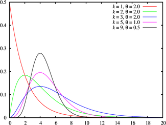 |
|
Cumulative distribution function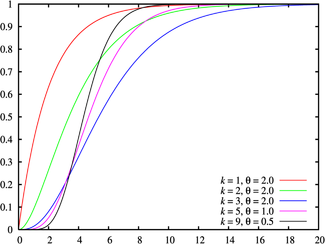 |
|
| Parameters |  shape (real) shape (real) scale (real) scale (real) |
|---|---|
| Support |  |
| Probability density function (pdf) |  |
| Cumulative distribution function (cdf) |  |
| Mean |  |
| Median | no simple closed form |
| Mode |  |
| Variance |  |
| Skewness |  |
| Excess kurtosis |  |
| Entropy |   |
| Moment-generating function (mgf) |  |
| Characteristic function |  |
In probability theory and statistics, the gamma distribution is a two-parameter family of continuous probability distributions. It has a scale parameter θ and a shape parameter k. If k is an integer then the distribution represents the sum of k independent exponentially distributed random variables, each of which has a mean of θ (which is equivalent to a rate parameter of θ −1) .
The gamma distribution is frequently a probability model for waiting times; for instance, in life testing, the waiting time until death is a random variable which is frequently modeled with a gamma distribution.[1]
Contents |
[edit] Characterization
A random variable X that is gamma-distributed with scale θ and shape k is denoted

[edit] Probability density function
The probability density function of the gamma distribution can be expressed in terms of the gamma function parameterized in terms of a shape parameter k and scale parameter θ. Both k and θ will be positive values.
The equation defining the probability density function of a gamma-distributed random variable x is
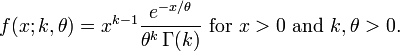
(This parameterization is used in the infobox and the plots.)
Alternatively, the gamma distribution can be parameterized in terms of a shape parameter α = k and an inverse scale parameter β = 1/θ, called a rate parameter:

If α is a positive integer, then

Both parameterizations are common because either can be more convenient depending on the situation.

[edit] Cumulative distribution function
The cumulative distribution function is the regularized gamma function, which can be expressed in terms of the incomplete gamma function,

It can also be expressed as follows, if k is an integer (i.e., the distribution is an Erlang distribution)[2]:

where β = 1/θ.
[edit] Properties
[edit] Summation
If Xi has a Γ(ki, θ) distribution for i = 1, 2, ..., N, then
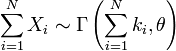
provided all Xi' are independent.
The gamma distribution exhibits infinite divisibility.
[edit] Scaling
For any t > 0 it holds that tX is distributed Γ(k, tθ), demonstrating that θ is a scale parameter.
[edit] Exponential family
The Gamma distribution is a two-parameter exponential family with natural parameters k − 1 and −1/θ, and natural statistics X and ln (X).
[edit] Information entropy
The information entropy is given by
![\frac{-1}{\theta^k \Gamma(k)} \int_0^{\infty} \frac{x^{k-1}}{e^{x/\theta}} \left[ (k-1)\ln x - x/\theta - k \ln\theta - \ln\Gamma(k) \right] \,dx \!](http://upload.wikimedia.org/math/a/d/8/ad87ea855f71036f04a153cac1f6fb12.png)
![= -\left[ (k-1) (\ln\theta + \psi(k)) - k - k \ln\theta - \ln\Gamma(k) \right] \!](http://upload.wikimedia.org/math/3/f/c/3fc6387b0016359b5150ea2a11b18df4.png)

where ψ(k) is the digamma function.

[edit] Kullback–Leibler divergence
The directed Kullback–Leibler divergence between Γ(α0, β0) ('true' distribution) and Γ(α, β) ('approximating' distribution) is given by

[edit] Laplace transform
The Laplace transform of the gamma PDF is

[edit] Parameter estimation
[edit] Maximum likelihood estimation
The likelihood function for N iid observations (x1, ..., xN) is

from which we calculate the log-likelihood function

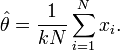
Finding the maximum with respect to θ by taking the derivative and setting it equal to zero yields the maximum likelihood estimator of the θ parameter:
Substituting this into the log-likelihood function gives

Finding the maximum with respect to k by taking the derivative and setting it equal to zero yields

where
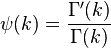
is the digamma function.
There is no closed-form solution for k. The function is numerically very well behaved, so if a numerical solution is desired, it can be found using, for example, Newton's method. An initial value of k can be found either using the method of moments, or using the approximation

If we let

then k is approximately

which is within 1.5% of the correct value.[citation needed] An explicit form for the Newton-Raphson update of this initial guess is given by Choi and Wette (1969) as the following expression:

where  denotes the trigamma function (the derivative of the digamma function).
The digamma and trigamma functions can be difficult to calculate with high precision. However, approximations known to be good to several significant figures can be computed using the following approximation formulae:

and

For details, see Choi and Wette (1969).
[edit] Bayesian minimum mean-squared error
With known k and unknown θ, the posterior PDF for theta (using the standard scale-invariant prior for θ) is

Denoting

Integration over θ can be carried out using a change of variables, revealing that 1/θ is gamma-distributed with parameters  .
.

The moments can be computed by taking the ratio (m by m = 0)
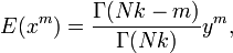
which shows that the mean +/- standard deviation estimate of the posterior distribution for theta is
 +/-
+/- 
[edit] Generating gamma-distributed random variables
Given the scaling property above, it is enough to generate gamma variables with θ = 1 as we can later convert to any value of β with simple division.
Using the fact that a Γ(1, 1) distribution is the same as an Exp(1) distribution, and noting the method of generating exponential variables, we conclude that if U is uniformly distributed on (0, 1], then −ln(U) is distributed Γ(1, 1). Now, using the "α-addition" property of gamma distribution, we expand this result:

where Uk are all uniformly distributed on (0, 1] and independent.
All that is left now is to generate a variable distributed as Γ(δ, 1) for 0 < δ < 1 and apply the "α-addition" property once more. This is the most difficult part.
We provide an algorithm without proof. It is an instance of the acceptance-rejection method:
- Let m be 1.
- Generate V3m − 2, V3m − 1 and V3m — independent uniformly distributed on (0, 1] variables.
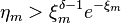
- If
 , where
  , then go to step 4, else go to step 5.
 - Let
 . Go to step 6.
 - Let
 .
. - If
 , then increment m and go to step 2.
 - Assume ξ = ξm to be the realization of Γ(δ,1)
Now, to summarize,
![\theta \left( \xi - \sum _{i=1} ^{[k]} {\ln U_i} \right) \sim \Gamma (k, \theta),](http://upload.wikimedia.org/math/c/4/e/c4ed98f33c39f06dc39ba1b97641876f.png)
where [k] is the integral part of k, and ξ has been generated using the algorithm above with δ = {k} (the fractional part of k), Uk and Vl are distributed as explained above and are all independent.
The GNU Scientific Library has robust routines for sampling many distributions including the Gamma distribution.
[edit] Related distributions
[edit] Specializations
- If
 , then X has an exponential distribution with rate parameter λ.
 - If
 , then X is identical to χ2(ν), the chi-square distribution with ν degrees of freedom.
 - If k is an integer, the gamma distribution is an Erlang distribution and is the probability distribution of the waiting time until the k-th "arrival" in a one-dimensional Poisson process with intensity 1/θ.
- If
 , then X has a Maxwell-Boltzmann distribution with parameter a.
  , then
[edit] Others
- If X has a Γ(k, θ) distribution, then 1/X has an inverse-gamma distribution with parameters k and θ-1.
- If X and Y are independently distributed Γ(α, θ) and Γ(β, θ) respectively, then X / (X + Y) has a beta distribution with parameters α and β.
- If Xi are independently distributed Γ(αi,θ) respectively, then the vector (X1 / S, ..., Xn / S), where S = X1 + ... + Xn, follows a Dirichlet distribution with parameters α1, ..., αn.
- For large k the gamma distribution converges to Gaussian distribution with mean μ = kθ and variance σ2 = kθ2.
- The Gamma distribution is the conjugate prior for the precision of the normal distribution with known mean.
- The Wishart distribution is a multivariate generalization of the Gamma distribution (samples are positive-definite matrices rather than positive real numbers).
[edit] Applications
| This section requires expansion. |
[edit] See also
| The Wikibook Statistics has a page on the topic of |
[edit] Notes
- ^ See Hogg and Craig Remark 3.3.1. for an explicit motivation.test
- ^ Papoulis, Pillai, Probability, Random Variables, and Stochastic Processes, Fourth Edition
[edit] References
- R. V. Hogg and A. T. Craig. Introduction to Mathematical Statistics, 4th edition. New York: Macmillan, 1978. (See Section 3.3.)
- Eric W. Weisstein, Gamma distribution at MathWorld.
- Engineering Statistics Handbook
- S. C. Choi and R. Wette. (1969) Maximum Likelihood Estimation of the Parameters of the Gamma Distribution and Their Bias, Technometrics, 11(4) 683–690


![[1]](http://commons.wikimedia.org/wiki/File:Gamma-PDF-3D-by-k.png)
![[2]](http://commons.wikimedia.org/wiki/File:Gamma-PDF-3D-by-Theta.png)
![[3]](http://commons.wikimedia.org/wiki/File:Gamma-PDF-3D-by-x.png)