Gradient descent

From Wikipedia, the free encyclopedia

Gradient descent is a first-order optimization algorithm. To find a local minimum of a function using gradient descent, one takes steps proportional to the negative of the gradient (or the approximate gradient) of the function at the current point. If instead one takes steps proportional to the gradient, one approaches a local maximum of that function; the procedure is then known as gradient ascent.

Gradient descent is also known as steepest descent, or the method of steepest descent. When known as the latter, gradient descent should not be confused with the method of steepest descent for approximating integrals.

[edit] Description

Gradient descent is based on the observation that if the real-valued function is defined and differentiable in a neighborhood of a point , then decreases fastest if one goes from in the direction of the negative gradient of F at , . It follows that, if

for γ > 0 a small enough number, then 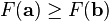. With this observation in mind, one starts with a guess for a local minimum of F, and considers the sequence such that

We have

so hopefully the sequence converges to the desired local minimum. Note that the value of the step size γ is allowed to change at every iteration.

This process is illustrated in the picture to the right. Here F is assumed to be defined on the plane, and that its graph has a bowl shape. The blue curves are the contour lines, that is, the regions on which the value of F is constant. A red arrow originating at a point shows the direction of the negative gradient at that point. Note that the (negative) gradient at a point is orthogonal to the contour line going through that point. We see that gradient descent leads us to the bottom of the bowl, that is, to the point where the value of the function F is minimal.

[edit] Examples

Gradient descent has problems with pathological functions such as the Rosenbrock function shown here. The Rosenbrock function has a narrow curved valley which contains the minimum. The bottom of the valley is very flat. Because of the curved flat valley the optimization is zig-zagging slowly with small stepsizes towards the minimum.

The gradient ascent method applied to :

[edit] Comments

Gradient descent works in spaces of any number of dimensions, even in infinite-dimensional ones. In the latter case the search space is typically a function space, and one calculates the Gâteaux derivative of the functional to be minimized to determine the descent direction.

Two weaknesses of gradient descent are:

1. The algorithm can take many iterations to converge towards a local minimum, if the curvature in different directions is very different.
2. Finding the optimal γ per step can be time-consuming. Conversely, using a fixed γ can yield poor results. Methods based on Newton's method and inversion of the Hessian using conjugate gradient techniques are often a better alternative.

A more powerful algorithm is given by the BFGS method which consists in calculating on every step a matrix by which the gradient vector is multiplied to go into a "better" direction, combined with a more sophisticated line search algorithm, to find the "best" value of γ.

Gradient descent is in fact Euler's method for solving ordinary differential equations applied to a gradient flow. As the goal is to find the minimum, not the flow line, the error in finite methods is less significant.

[edit] A computational example

The gradient descent algorithm is applied to find a local minimum of the function f(x)=x⁴-3x³+2 , with derivative f'(x)=4x³-9x². Here is an implementation in the C programming language.

#include <stdio.h>
#include <stdlib.h>
#include <math.h>
 
int main ()
{
	// From calculation, we expect that the local minimum occurs at x=9/4
	// The algorithm starts at x=6
 
	double xOld = 0;
	double xNew = 6;
	double eps = 0.01; // step size
	double precision = 0.00001;
	while (fabs(xNew - xOld) > precision)
	{
             xOld = xNew;
             xNew = xNew - eps*(4*xNew*xNew*xNew-9*xNew*xNew);
	}
 
	printf ("Local minimum occurs at %lg\n", xNew);
 
}

With this precision, the algorithm converges to a local minimum of 2.24996 in 70 iterations.

A more robust implementation of the algorithm would also check whether the function value indeed decreases at every iteration and would make the step size smaller otherwise. One can also use an adaptive step size which may make the algorithm converge faster.

[edit] See also

[edit] References

• Mordecai Avriel (2003). Nonlinear Programming: Analysis and Methods. Dover Publishing. ISBN 0-486-43227-0.
• Jan A. Snyman (2005). Practical Mathematical Optimization: An Introduction to Basic Optimization Theory and Classical and New Gradient-Based Algorithms. Springer Publishing. ISBN 0-387-24348-8