Lagrange polynomial

From Wikipedia, the free encyclopedia

In numerical analysis, a Lagrange polynomial, named after Joseph Louis Lagrange, is the interpolating polynomial for a given set of data points in the Lagrange form. It was first discovered by Edward Waring in 1779 and later rediscovered by Leonhard Euler in 1783.

As there is only one interpolation polynomial for a given set of data points it is a bit misleading to call the polynomial the Lagrange interpolation polynomial. The more precise name is the Lagrange form of the interpolation polynomial.

This image shows, for four points ((−9, 5), (−4, 2), (−1, −2), (7, 9)), the (cubic) interpolation polynomial L(x), which is the sum of the scaled basis polynomials y₀ℓ₀(x), y₁ℓ₁(x), y₂ℓ₂(x) and y₃ℓ₃(x). The interpolation polynomial passes through all four control points, and each scaled basis polynomial passes through its respective control point and is 0 where x corresponds to the other three control points.

[edit] Definition

Given a set of k + 1 data points

$(x_0, y_0),\ldots,(x_k, y_k)$

where no two x_j are the same, the interpolation polynomial in the Lagrange form is a linear combination

$L(x) := \sum_{j=0}^{k} y_j \ell_j(x)$

of Lagrange basis polynomials

$\ell_j(x) := \prod_{i=0,\, i\neq j}^{k} \frac{x-x_i}{x_j-x_i} = \frac{(x-x_0)}{(x_j-x_0)} \cdots \frac{(x-x_{j-1})}{(x_j-x_{j-1})} \frac{(x-x_{j+1})}{(x_j-x_{j+1})} \cdots \frac{(x-x_{k})}{(x_j-x_{k})}.$

[edit] Proof

The function we are looking for has to be a polynomial function L(x) of degree less than or equal to k with

$L(x_j) = y_j \qquad j=0,\ldots,k$

The Lagrange polynomial is a solution to the interpolation problem.

As can be seen

$\ell_j(x)$ is a polynomial and has degree k.
$\ell_i(x_j) = \delta_{ij},\quad 0 \leq i,j \leq k.\,$

Thus the function L(x) is a polynomial with degree at most k and

$L(x_i) = \sum_{j=0}^{k} y_j \ell_j(x_i) = \sum_{j=0}^{k} y_j \delta_{ji} = y_i.$

There can be only one solution to the interpolation problem since the difference of two such solutions would be a polynomial with degree at most k and k+1 zeros. This is only possible if the difference is identically zero, so L(x) is the unique polynomial interpolating the given data.

[edit] Main idea

Solving an interpolation problem leads to a problem in linear algebra where we have to solve a matrix. Using a standard monomial basis for our interpolation polynomial we get the very complicated Vandermonde matrix. By choosing another basis, the Lagrange basis, we get the much simpler identity matrix = δ_i,j which we can solve instantly.

[edit] Implementation in C

Note : "pos" and "val" arrays are of size "degree".

float lagrangeInterpolatingPolynomial (float pos[], float val[], int degree, float desiredPos)  { 
   float retVal = 0; 
 
   for (int i = 0; i < degree; ++i) { 
      float weight = 1; 
 
      for (int j = 0; j < degree; ++j) {
         // The i-th term has to be skipped
         if (j != i) {
            weight *= (desiredPos - pos[j]) / (pos[i] - pos[j]);
         }
      }
 
      retVal += weight * val[i]; 
   } 
 
   return retVal; 
}

[edit] Usage

[edit] Example 1

The tangent function and its interpolant

Find an interpolation formula for $f (x) = tan(x)$ given this set of known values:

$x_0=-1.5\,$	$f(x_0)=-14.1014\,$
$x_1=-0.75\,$	$f(x_1)=-0.931596\,$
$x_2=0\,$	$f(x_2)=0\,$
$x_3=0.75\,$	$f(x_3)=0.931596\,$
$x_4=1.5\,$	$f(x_4)=14.1014.\,$

The basis polynomials are:

$\ell_0(x)={x - x_1 \over x_0 - x_1}\cdot{x - x_2 \over x_0 - x_2}\cdot{x - x_3 \over x_0 - x_3}\cdot{x - x_4 \over x_0 - x_4} ={1\over 243} x (2x-3)(4x-3)(4x+3)$

$\ell_1(x) = {x - x_0 \over x_1 - x_0}\cdot{x - x_2 \over x_1 - x_2}\cdot{x - x_3 \over x_1 - x_3}\cdot{x - x_4 \over x_1 - x_4} = {} -{8\over 243} x (2x-3)(2x+3)(4x-3)$

$\ell_2(x)={x - x_0 \over x_2 - x_0}\cdot{x - x_1 \over x_2 - x_1}\cdot{x - x_3 \over x_2 - x_3}\cdot{x - x_4 \over x_2 - x_4} ={3\over 243} (2x+3)(4x+3)(4x-3)(2x-3)$

$\ell_3(x)={x - x_0 \over x_3 - x_0}\cdot{x - x_1 \over x_3 - x_1}\cdot{x - x_2 \over x_3 - x_2}\cdot{x - x_4 \over x_3 - x_4} =-{8\over 243} x (2x-3)(2x+3)(4x+3)$

$\ell_4(x)={x - x_0 \over x_4 - x_0}\cdot{x - x_1 \over x_4 - x_1}\cdot{x - x_2 \over x_4 - x_2}\cdot{x - x_3 \over x_4 - x_3} ={1\over 243} x (2x+3)(4x-3)(4x+3).$

Thus the interpolating polynomial then is

$\begin{align}L(x) &= {1\over 243}\Big(f(x_0)x (2x-3)(4x-3)(4x+3) \\ & {} - 8f(x_1)x (2x-3)(2x+3)(4x-3) \\ & {} + 3f(x_2)(2x+3)(4x+3)(4x-3)(2x-3) \\ & {} - 8f(x_3)x (2x-3)(2x+3)(4x+3) \\ & {} + f(x_4)x (2x+3)(4x-3)(4x+3)\Big)\\ & = 4.834848x^3 - 1.477474x. \end{align}$

[edit] Example 2

We wish to interpolate ƒ(x) = x² over the range 1 ≤ x ≤ 3, given these 3 points:

$x_0=1\,$	$f(x_0)=1\,$
$x_1=2\,$	$f(x_1)=4\,$
$x_2=3\,$	$f(x_2)=9.\,$

The interpolating polynomial is:

$\begin{align} L(x) &= {1}\cdot{x - 2 \over 1 - 2}\cdot{x - 3 \over 1 - 3}+{4}\cdot{x - 1 \over 2 - 1}\cdot{x - 3 \over 2 - 3}+{9}\cdot{x - 1 \over 3 - 1}\cdot{x - 2 \over 3 - 2} \\ &= x^2. \end{align}$

[edit] Example 3

We wish to interpolate ƒ(x) = x³ over the range 1 ≤ x ≤ 3, given these 3 points:

$x_0=1\,$	$f(x_0)=1\,$
$x_1=2\,$	$f(x_1)=8\,$
$x_2=3\,$	$f(x_2)=27\,$

The interpolating polynomial is:

$\begin{align} L(x) &= {1}\cdot{x - 2 \over 1 - 2}\cdot{x - 3 \over 1 - 3}+{8}\cdot{x - 1 \over 2 - 1}\cdot{x - 3 \over 2 - 3}+{27}\cdot{x - 1 \over 3 - 1}\cdot{x - 2 \over 3 - 2} \\ &= 6x^2 - 11x + 6. \end{align}$

[edit] Notes

The Lagrange form of the interpolation polynomial shows the linear character of polynomial interpolation and the uniqueness of the interpolation polynomial. Therefore, it is preferred in proofs and theoretical arguments. But, as can be seen from the construction, each time a node x_k changes, all Lagrange basis polynomials have to be recalculated. A better form of the interpolation polynomial for practical (or computational) purposes is the barycentric form of the Lagrange interpolation (see below) or Newton polynomials.

Lagrange and other interpolation at equally spaced points, as in the example above, yield a polynomial oscillating above and below the true function. This behaviour tends to grow with the number of points, leading to a divergence known as Runge's phenomenon; the problem may be eliminated by choosing interpolation points at Chebyshev nodes.

The Lagrange basis polynomials can be used in numerical integration to derive the Newton–Cotes formulas.

[edit] Barycentric interpolation

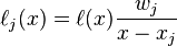
Using the quantity

$\ell(x) = (x - x_0)(x - x_1) \cdots (x - x_k)$

we can rewrite the Lagrange basis polynomials as

$\ell_j(x) = \frac{\ell(x)}{x-x_j} \frac{1}{\prod_{i=0,i \neq j}^k(x_j-x_i)}$

or, by defining the barycentric weights^[1]

$w_j = \frac{1}{\prod_{i=0,i \neq j}^k(x_j-x_i)}$

we can simply write

$\ell_j(x) = \ell(x)\frac{w_j}{x-x_j}$

which is commonly referred to as the first form of the barycentric interpolation formula.

The advantage of this representation is that the interpolation polynomial may now be evaluated as

$L(x) = \ell(x) \sum_{j=0}^k \frac{w_j}{x-x_j}y_j$

which, if the weights $w j$ have been pre-computed, requires only $\mathcal O(n)$ operations (evaluating $\ell(x)$ and the weights $w j / (x - x j)$ ) as opposed to $\mathcal O(n^2)$ for evaluating the Lagrange basis polynomials $\ell_j(x)$ individually.

The barycentric interpolation formula can also easily be updated to incorporate a new node $x k + 1$ by dividing each of the $w j$ , $j=0 \dots k$ by $(x j - x k + 1)$ and constructing the new $w k + 1$ as above.

We can further simplify the first form by first considering the barycentric interpolation of the constant function $g(x)\equiv 1$ :

$g(x) = \ell(x) \sum_{j=0}^k \frac{w_j}{x-x_j}.$

Dividing $L (x)$ by $g (x)$ does not modify the interpolation, yet yields

$L(x) = \frac{\sum_{j=0}^k \frac{w_j}{x-x_j}y_j}{\sum_{j=0}^k \frac{w_j}{x-x_j}}$

which is referred to as the second form or true form of the barycentric interpolation formula. This second form has the advantage, that $\ell(x)$ need not be evaluated for each evaluation of $L (x)$ .

[edit] See also

Polynomial interpolation
Newton form of the interpolation polynomial
Bernstein form of the interpolation polynomial
Newton–Cotes formulas

[edit] External links

[edit] References

^ Jean-Paul Berrut, Lloyd N. Trefethen (2004) "Barycentric Lagrange Interpolation" in SIAM Review Volume 46 (3), pages 501–517. DOI:10.1137/S0036144502417715
^ Zachary Battles, Lloyd N. Trefethen (2004) "An Extension of Matlab to Continuous Functions and Operators" in SIAM J. Sci. Comput. Volume 25 (5), pages 1743–1770. DOI:10.1137/S1064827503430126

[0] Jean-Paul Berrut, Lloyd N. Trefethen (2004) "Barycentric Lagrange Interpolation" in SIAM Review Volume 46 (3), pages 501–517. DOI:10.1137/S0036144502417715

[1] Zachary Battles, Lloyd N. Trefethen (2004) "An Extension of Matlab to Continuous Functions and Operators" in SIAM J. Sci. Comput. Volume 25 (5), pages 1743–1770. DOI:10.1137/S1064827503430126

[1]

[2]

Lagrange polynomial

From Wikipedia, the free encyclopedia

Contents

[edit] Definition

[edit] Proof

[edit] Main idea

[edit] Implementation in C

[edit] Usage

[edit] Example 1

[edit] Example 2

[edit] Example 3

[edit] Notes

[edit] Barycentric interpolation

[edit] See also

[edit] External links

[edit] References

Views

Personal tools

Navigation

Search

Interaction

Toolbox

Languages