Kernel density estimation
From Wikipedia, the free encyclopedia
In statistics, kernel density estimation (or Parzen window method, named after Emanuel Parzen) is a non-parametric way of estimating the probability density function of a random variable. As an illustration, given some data about a sample of a population, kernel density estimation makes it possible to extrapolate the data to the entire population.
The Parzen window is also used in signal processing as a lag window, in such procedures as the Blackman-Tukey procedure.
A histogram can be thought of as a collection of point samples from a kernel density estimate for which the kernel is a uniform box the width of the histogram bin.
Contents |
[edit] Definition
If x1, x2, ..., xN ~ ƒ is an independent and identically-distributed sample of a random variable, then the kernel density approximation of its probability density function is

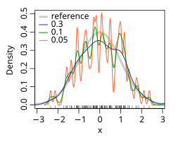
where K is some kernel and h is a smoothing parameter called the bandwidth. Quite often K is taken to be a standard Gaussian function with mean zero and variance 1:[dubious ]

[edit] Intuition
Although less smooth density estimators such as the histogram density estimator can be made to be asymptotically consistent, others are often either discontinuous or converge at slower rates than the kernel density estimator. Rather than grouping observations together in bins, the kernel density estimator can be thought to place small "bumps" at each observation, determined by the kernel function. The estimator consists of a "sum of bumps" and is clearly smoother as a result (see below image).

[edit] Properties
Let  be the L2 risk function for ƒ. Under weak assumptions on ƒ and K,

By minimizing the theoretical risk function, it can be shown that the optimal bandwidth is

where


When the optimal choice of bandwidth is chosen, the risk function is  for some constant c4 > 0. It can be shown that, under weak assumptions, there cannot exist a non-parametric estimator that converges at a faster rate than the kernel estimator. Note that the n−4/5 rate is slower than the typical n−1 convergence rate of parametric methods.
It is possible to optimize the bandwidth by leave-one-out cross validation.[1]
[edit] Statistical implementation
- In Matlab, kernel density estimation is implemented through the
ksdensityfunction, but this function does not provide automatic data-driven bandwidth. A free Matlab software which implements an automatic bandwidth selection method is available from the Matlab repository [1] for 1 dimensional data and [2] for 2 dimensional data. - An example of implementing kernel density estimation in Mathematica is available here.
- In Stata, it is implemented through
kdensity; for examplehistogram x, kdensity. - In R, it is implemented through the
densityfunction (univariate), thekde2dfunction in theMASSpackage (bivariate), and thenpudensfunction in the np package (multivariate allowing for numeric and categorical data types with a range of kernel functions and automatic bandwidth selectors). - In SAS,
proc kdecan be used to estimate univariate and bivariate kernel densities. - In SciPy,
scipy.stats.gaussian_kdecan be used to perform gaussian kernel density estimation in arbitrary dimensions, including bandwidth estimation. - In Perl, an implementation can be found in the Statistics-KernelEstimation module [3]
- In Java, the Weka (machine learning) package provides weka.estimators.KernelEstimator[4], among others.
- In Gnuplot, kernel desity esimation is implemented by the
smooth kdensityoption, the datafile can contain weigth and bandwidth for each point, or the bandwidth can be set automatically.
[edit] Example of Density Estimation in R programming language
This example is based on the Old Faithful Geyser, a tourist attraction located in Yellowstone National Park. This famous dataset containing 272 records consists of two variables, eruption duration (minutes) and waiting time until the next eruption (minutes). The data is taken from the datasets package of the R programming language.
We consider estimating the joint density of eruption duration and waiting times using the R np package that employs automatic (data-driven) bandwidth selection that is optimal for joint density estimates; see the np vignette for an introduction to the np package. The figure below shows the joint density estimate using a second order Gaussian kernel.

[edit] Script for example
The following commands of the R programming language use the npudens() function to deliver optimal smoothing and to create the figure given above. These commands can be entered at the command prompt by using cut and paste.
library(np)
library(datasets)
data(faithful)

f <- npudens(~eruptions+waiting,data=faithful)

plot(f,view="fixed",neval=100,phi=30,main="",xtrim=-0.2)
[edit] See also
- Kernel (statistics)
- Kernel (mathematics)
- Kernel smoothing
- Mean-shift
- Scale space (The surface in x, bandwidth, Density space for all bandwidths is essentially a scale space representation of the data.)
[edit] External links
- Introduction to kernel density estimation
- Free Matlab m-file for one and two dimensional kernel density estimation
- Free Online Software (Calculator) computes the Kernel Density Estimation for any data series according to the following Kernels: Gaussian, Epanechnikov, Rectangular, Triangular, Biweight, Cosine, and Optcosine.
- FIGTree is a fast library that can be used to compute Kernel Density Estimates using a Gaussian Kernel. MATLAB and C/C++ interfaces available.
- Good summary of methods to choose bandwidth Bandwidth Selection in Kernel Density Estimation: A Review.
- The np package An R package that provides a variety of nonparametric and semiparametric kernel methods that seamlessly handle a mix of continuous, unordered, and ordered factor data types.
- Kernel Density Estimation Applet An online interactive example of kernel density estimation. Requires .NET 3.0 or later.
- Mathematica KDE demo An interactive demo in Mathematica that can be explored using the free player.
[edit] References
- ^ Finn Årup Nielsen; Lars Kai Hansen (March 2002). "Modeling of activation data in the BrainMapTM: Detection of outliers". Human Brain Mapping 15 (3): 146–156. doi:. PMID 11835605. http://www2.imm.dtu.dk/pubdb/views/publication_details.php?id=197.
- Li, Q. and Racine, J.S. Nonparametric Econometrics: Theory and Practice. Princeton University Press, 2007, ISBN 0691121613.
- Parzen E. (1962). On estimation of a probability density function and mode, Ann. Math. Stat. 33, pp. 1065–1076.
- Duda, R. and Hart, P. (1973). Pattern Classification and Scene Analysis. John Wiley & Sons. ISBN 0-471-22361-1.
- Wasserman, L. (2005). All of Statistics: A Concise Course in Statistical Inference, Springer Texts in Statistics.

