basictheories development economics environment incomebooklet metode2 simon_kuznets socialecology theory water waterworldresearch

My tags:

From Wikipedia, the free encyclopedia

This article may need to be rewritten entirely to comply with Wikipedia's quality standards. You can help. The discussion page may contain suggestions.

This article does not cite any references or sources. Please help improve this article by adding citations to reliable sources (ideally, using inline citations). Unsourced material may be challenged and removed. (December 2007)

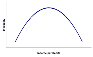
Kuznets curve is the graphical representation of Simon Kuznets's theory ('Kuznets hypothesis') that economic inequality increases over time while a country is developing, then after a critical average income is attained, begins to decrease.

One theory as to why this happens states that in early stages of development, when investment in physical capital is the main mechanism of economic growth, inequality encourages growth by allocating resources towards those who save and invest the most. Whereas in mature economies human capital accrual, or an estimate of cost that has been incurred but not yet paid, takes the place of physical capital accrual as the main source of growth, and inequality slows growth by lowering education standards because poor people lack finance for their education in imperfect credit markets. Kuznets curve diagrams show an inverted U curve, although variables along the axes are often mixed and matched, with inequality or the Gini coefficent on the Y axis and economic development, time or per capita incomes on the X axis.

Contents 1 Kuznets ratio 2 Interpretation 3 Criticism 4 Environmental Kuznets Curve 5 See also 6 References 7 Sources and bibliography

[edit] Kuznets ratio

The Kuznets ratio is a measurement of the ratio of income going to the highest-earning households (usually defined by the upper 20%) and the income going to the lowest-earning households, which is commonly measured by either the lowest 20% or lowest 40% of income. Comparing 20% to 20%, perfect equality is expressed as 1; 20% to 40% changes this value to 0.5.

Kuznets had two similar explanations for this historical phenomenon:

• workers migrated from agriculture to industry,
• rural workers moved to urban jobs.

In both explanations, inequality will decrease after 50% of the work force switches over to the higher paying sector. Economic historians have since used skill gap theories and the theories of capital concentration in early economies from classical economists and Marxists to further explain the Kuznets curve.

[edit] Interpretation

Kuznets Curve can be interpreted as follows. The transition from an agrarian sector to urban industrialization, in which we see a growth in income inequality as income in agriculture is relatively low compared to income earned in the city. With this opening up of inequality, we also see that the level of income people earn in rural areas is similar to one another, whereas we see wide range of income level in the industrialized city, which further opens up inequality. What then generates decline in Kuznets Curve? First, a rise of mass education movement may open up opportunity for all and reduce the gap in income inequality. Second, social policy put forth by the government as a country becomes rich may explain a decline in inequality as the government provides transfers, welfare, retirement pension, health care, in an effort to redistribute income throughout different levels of income earning groups.

In the case of the United States, we can model income inequality through Kuznets Curve with underlying mechanisms such as education and government redistribution which seem to generate up and down concave shaped curves. We can see from the sources presented by Alice Hansen Jones (1775); Edward Wolff (1915-1995) the share of wealth held by the top 1% from 1775 to 1995. Around 1775, the top 1% owned about 15% of the wealth, then 30% by 1855 according to the U.S Census. The data presented shows inequality to peak around 1935, with the top 1% owning 45% of the share of wealth in the United States and then begin a decline toward the civil-war era levels from the World War II years to the 1970s. This period of decline occurred during Kuznets' lifetime and appears to be consistent with his theory regarding inequality. However, there has since been a steady increase in the share of wealth held by the top 1%. By the 1990s, inequality had climbed back to late-1930s levels. One possible explanation for this divergence from the Kuznets' curve is the impact of American social mobility on wealth distribution. Kuznets believed that as a country grew richer, its government would make a greater effort towards social spending. But in the U.S., high social mobility fostered a belief in the rewards of "hard work," which, in turn, may have resulted in more employer-provided social programs (welfare capitalism) and less of a welfare state.

[edit] Criticism

Kuznets' conclusion that inequality must increase before decreasing, however, rests on shaky ground, in the case of cross-sectional data. The U-shape in the curve comes not from progression in the development of individual countries, but rather from historical differences between countries. In his data set, many of the middle income countries were in Latin America, a region with historically high levels of inequality. When controlling for this variable, the U-shape of the curve tends to disappear. In accounting for historical changes, David Lempert's work in the early 1980s introduced a time dimension and a political dimension to the curve, showing how population and politics interact with economic inequality over time, leading either to long-term stability or to collapse. This neo-Malthusian model incorporating Kuznets' work, yields a helix model of the relationships over time rather than just a curve. ^[1]

[edit] Environmental Kuznets Curve

Another situation where the Kuznets curve is alleged to appear is the environment. Many environmental health indicators, such as water and air pollution, show the inverted U-shaped curve. The argument for the environmental Kuznet's curve is based on the following argument. In a developing industrial economy, little weight is given to environmental concerns, raising environmental pollution byproducts. After attaining a certain standard of living from the industrial production system and when environmental pollution is at its greatest, the focus changes from self-interest to social interest. The interests give greater weight to a clean environment by reducing and reversing the environmental pollution trend from industrialization. This parabolic trend occurs in the level of many of the environmental pollutants, such as sulfur dioxide, nitrogen oxide, lead, DDT, chlorofluorocarbons, sewage, and other chemicals previously released directly into the air or water.

For example, between 1970 and 2006, the United States' inflation-adjusted GDP grew by 195%, the number of cars and trucks in the country more than doubled, and the total number of miles driven increased by 178%. However, during that same time period, annual emissions of carbon monoxide fell from 197 million tons to 89 million, nitrogen oxides emissions fell from 27 million tons to 19 million, sulfur dioxide emissions fell from 31 million tons to 15 million, particulate emissions fell by 80%, and lead emissions fell by more than 98%. ^[2]

However, there is little evidence that the relationship holds true for other pollutants, for natural resource use or for biodiversity conservation. For example, energy, land and resource use (sometimes called the "ecological footprint") do not fall with rising income. While the ratio of energy per real GDP has fallen, total energy use is still rising in most developed countries. Another example is the emission of many greenhouse gases, which is much higher in industrialised countries. In addition, the status of many key "ecosystem services" provided by ecosystems, such as freshwater provision and regulation,(Perman, et al., 2003) soil fertility,^{[citation needed]} and fisheries,^{[citation needed]} have continued to decline in developed countries. In general, Kuznets curves have been found for some environmental health concerns (such as air pollution) but not for others (such as landfills and biodiversity). However, it is important to note that this does not necessarily invalidate the theory - the scale of the Kuznets curves may differ for different environmental impacts. We may still be on the 'upward' leg of the energy use Kuznets curve and have to get even richer still before we see a decline. If so, however, we are causing many irreversible environmental impacts in the process. Also, many of the problems associated with increased energy usage are due to the use of fossil fuels. Alternatives such as nuclear power and renewable energy would have a much lower environmental impact according to their proponents. Against this must be considered that much of the environmental damage associated with economic growth, such as extinct species and loss of wilderness, is irreversible.

Carbon dioxide appears to follow a Kuznets curve, and its emissions appear to peak at a per capita GDP of approximately $30,000.^[3]

The problem of deforestation also appears to follow a Kuznets curve. Among countries with a per capita GDP of at least $4,600, net deforestation has ceased to exist. ^[4]

Rich countries are able to afford desalination to provide their populations with clean, safe water. Israel desalinizes water for a cost of 53 cents per cubic meter ^[5] Singapore desalinizes water for 49 cents per cubic meter ^[6]. Even people who live far away from the ocean are benefitting from the technology - after being desalinized at Jubail, Saudi Arabia, water is pumped 200 miles (320 km) inland though a pipeline to the capital city of Riyadh. ^[7]

The developing economy of China has been cited as a potential test case for the "environmental Kuznets Curve" (EKC).^[8]

It is important to realize that the initial hypothesis saw a decrease in pollutants at a threshold GDP of 8,000 dollars per capita. Some people argue that even the US is still struggling to attain the income level necessary to prioritize certain environmental pollutants such as carbon emissions, which have yet to follow the EKC ^[9]. With other pollutants however, like sulfur dioxide, production seems to coincide with a country's economic development and at a certain threshold level of income a mitigation of environmental damage occurs. This could be related rather causal, because economic growth without institutional reform does not accomplish this environmental improvement. It appears that with GDP growth, government policies are strengthened and populations experience a rise in their demand for improved environmental quality.

This could be a reason why the EKC has been found to be applicable to only certain types of pollutants.^[9] For example, the EKC has not been found to apply to carbon for a few reasons. Most pollutants create localized problems like lead and sulfur, so there is a greater urgency and response to cleaning up such pollutants. As a country develops, the marginal value of cleaning up such pollutants makes a relatively large direct improvement to the quality of citizens' lives. Conversely, reducing carbon dioxide emissions does not have a dramatic impact at a local level, so the impetus to clean them up is only for the altruistic reason of improving the global environment. This becomes a tragedy of the commons where it is most efficient for everyone to pollute and for no one to clean-up, and everyone is worse as a result (Hardin, 1968). Thus, even in a country like the US with a high level of income, carbon emissions are not decreasing in accordance with the EKC.^[9]

A recent theory that some researchers have been examining with the EKC is that the traditional "inverse U" shape is actually an "N" shape when longer-term time scales are evaluated. This "N" shape would indicate that pollution increases as a country develops, decreases once the threshold GDP is reached, and then begins increasing as national income continues to increase. While this finding is still being debated, it could prove to be important because it poses the concerning question of whether pollution actually begins to decline for good when an economic threshold is reached or whether the decrease is only in local pollutants and pollution is simply exported to poorer developing countries.^[10]

Economists have hypothesized that economic growth does not have to come as a result of increasing environmental degradation. This "N" shape could support their claim because, even in highly developed countries, pollution continues to increase at extremely high levels of income. This would indicate that pollution and economic growth are separate and only sometimes correlated. Hence, the traditional pollution-income progression of agrarian communities (clean) to industrial economies (pollution intensive) to service economies (cleaner) would appear to be false if pollution increases again at the end due to higher levels of income and consumption of the population at large (Arrow, et al., 1995). A difficulty with this model is that it lacks predictive power because it is highly uncertain how the next phase of economic development will be characterized.

A more significant problem with the original "U" shaped model is the troubling concern that a net pollution reduction may not actually be occurring on global scales. Wealthy nations have a trend of exporting the activities that create the most pollution, like manufacturing of clothing and furniture, to poorer nations that are still in the process of industrial development (Suri and Chapman, 1998). This means that as the world's poor nations develop, they will have no place to export their pollution. Thus, this progression of environmental cleanup occurring in conjunction with economic growth cannot be replicated indefinitely because there will be nowhere to export waste and pollution intensive processes. Even Grossman and Kruger (1995), the authors who initially made the correlation between economic growth, environmental clean-up, and the Kuznets curve, conclude that there is "no evidence that environmental quality deteriorates steadily with economic growth."^[10]

[edit] See also

• Clean growth

[edit] References

[edit] Sources and bibliography

• Grossman, G.M. and Krueger, A.B. (1993). Environmental Impacts of a North American Free Trade Agreement. In The Mexico-U.S. Free Trade Agreement, P. Garber, ed. Cambridge, Mass.: MIT Press.

• Shafik, N., “Economic Development and Environmental Quality: An Econometric Analysis”, Oxford Economic Papers, New Series, Vol. 46, Special Issue on Environmental Economics (Oct., 1994), pp. 757-773.

• Deacon, R.T. and C.S. Norman "Does the Environmental Kuznets Curve Describe How Individual Countries Behave?". Land Economics. vol.82. 2 (2006). pp. 291 - 315.

• Arrow, K., Bolin, B., Costanza, R., Dasgupta, P., Folke, C., Holling, C. S., et al. (1995). Economic growth, carrying capacity, and the environment. Ecological Economics, 15(2), 91-95.

• Brenner, Y.S., Hartmut Kaelble, and Mark Thomas (1991): Income Distribution in Historical Perspective. Cambridge University Press.

• Van Zanden, J.L. (1995). Tracing the Beginning of the Kuznets Curve: Western Europe during the Early Modern Period. The Economic History Review, 48(4), 643-664.

• Tisdell, C. (2001). Globalisation and sustainability: environmental Kuznets curve and the WTO. Ecological Economics, 39(2), 185-196.

• Dasgupta, S., Laplante, B., Wang, H. and Wheeler, D. (2002). Confronting the Environmental Kuznets Curve. The Journal of Economic Perspectives, 16(1), 147-168.

• Harbaugh, B., Levinson, A. and Wilson, D. (2002). Reexamining the Empirical Evidence for an Environmental Kuznets Curve. Review of Economics and Statistics, 84(3).

• Munir Khasru Syed, Muaz Jalil Mohammad (2004), Revisiting Kuznets Hypothesis: An Analysis with Time Series and Panel Data,Bangladesh Development Studies, Vol 30 No 3-4, pg 89-112

• Munir Khasru Syed, Muaz Jalil Mohammad (2004), Revisiting Kuznets Hypothesis: An Analysis with Time Series and Panel Data (Draft) http://papers.ssrn.com/sol3/papers.cfm?abstract_id=1240658

• Millennium Ecosystem Assessment (2005). "Ecosystems and Human Wellbeing: Synthesis" (pdf). Island Press. http://www.millenniumassessment.org/documents/document.356.aspx.pdf.