Window function
From Wikipedia, the free encyclopedia
- See also Window function (SQL)
In signal processing, a window function (also known as an apodization function or tapering function[1]) is a function that is zero-valued outside of some chosen interval. For instance, a function that is constant inside the interval and zero elsewhere is called a rectangular window, which describes the shape of its graphical representation. When another function or a signal (data) is multiplied by a window function, the product is also zero-valued outside the interval: all that is left is the "view" through the window. Applications of window functions include spectral analysis, filter design and beamforming.
A more general definition of window functions does not require them to be identically zero outside an interval, as long as the product of the window times its argument is square integrable, that is, that the function goes sufficiently rapidly toward zero.[2]
In typical applications, the window functions used are non-negative smooth "bell shaped" curves,[3] though rectangle and triangle functions and other functions are sometimes used.
[edit] Spectral analysis
The Fourier transform of the function:  is zero, except at frequency
  . However, many other functions and data (that is, waveforms) do not have convenient closed form transforms. Alternatively, one might be interested in their spectral content only during a certain time period.
In either case, the Fourier transform (or something similar) can be applied on one or more finite intervals of the waveform. In general, the transform is applied to the product of the waveform and a window function. Any window (including rectangular) affects the spectral estimate computed by this method.
[edit] Windowing
Windowing of a simple waveform, like causes its Fourier transform to have non-zero values (commonly called spectral leakage) at frequencies other than ω. It tends to be worst (highest) near ω and least at frequencies farthest from ω.
If there are two sinusoids, with different frequencies, leakage can interfere with the ability to distinguish them spectrally. If their frequencies are dissimilar, then the leakage interferes when one sinusoid is much smaller in amplitude than the other. That is, its spectral component can be hidden by the leakage from the larger component. But when the frequencies are near each other, the leakage can be sufficient to interfere even when the sinusoids are equal strength; that is, they become unresolvable.
The rectangular window has excellent resolution characteristics for signals of comparable strength, but it is a poor choice for signals of disparate amplitudes. This characteristic is sometimes described as low-dynamic-range.
At the other extreme of dynamic range are the windows with the poorest resolution. These high-dynamic-range low-resolution windows are also poorest in terms of sensitivity; this is, if the input waveform contains random noise close to the signal frequency, the response to noise, compared to the sinusoid, will be higher than with a higher-resolution window. In other words, the ability to find weak sinusoids amidst the noise is diminished by a high-dynamic-range window. High-dynamic-range windows are probably most often justified in wideband applications, where the spectrum being analyzed is expected to contain many different signals of various strengths.
In between the extremes are moderate windows, such as Hamming and Hann. They are commonly used in narrowband applications, such as the spectrum of a telephone channel. In summary, spectral analysis involves a tradeoff between resolving comparable strength signals with similar frequencies and resolving disparate strength signals with dissimilar frequencies. That tradeoff occurs when the window function is chosen.
[edit] Discrete-time signals
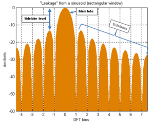
When the input waveform is time-sampled, instead of continuous, the analysis is usually done by applying a window function and then a discrete Fourier transform (DFT). But the DFT provides only a coarse sampling of the actual DTFT spectrum. Figure 1 shows a portion of the DTFT for a rectangularly-windowed sinusoid. The actual frequency of the sinusoid is indicated as "0" on the horizontal axis. Everything else is leakage. The unit of frequency is "DFT bins"; that is, the integer values on the frequency axis correspond to the frequencies sampled by the DFT. So the figure depicts a case where the actual frequency of the sinusoid happens to coincide with a DFT sample, and the maximum value of the spectrum is accurately measured by that sample. When it misses the maximum value by some amount [up to 1/2 bin], the measurement error is referred to as scalloping loss (inspired by the shape of the peak). But the most interesting thing about this case is that all the other samples coincide with nulls in the true spectrum. (The nulls are actually zero-crossings, which cannot be shown on a logarithmic scale such as this.) So in this case, the DFT creates the illusion of no leakage. Despite the unlikely conditions of this example, it is a popular misconception that visible leakage is some sort of artifact of the DFT. But since any window function causes leakage, its apparent absence (in this contrived example) is actually the DFT artifact.
[edit] Noise bandwidth
The concepts of resolution and dynamic range tend to be somewhat subjective, depending on what the user is actually trying to do. But they also tend to be highly correlated with the total leakage, which is quantifiable. It is usually expressed as an equivalent bandwidth, B. Think of it as redistributing the DTFT into a rectangular shape with height equal to the spectral maximum and width B. The more leakage, the greater the bandwidth. It is sometimes called noise equivalent bandwidth or equivalent noise bandwidth, because it is proportional to the average power that will be registered by each DFT bin when the input signal contains a random noise component (or is just random noise). A graph of the power spectrum, averaged over time, typically reveals a flat noise floor, caused by this effect. The height of the noise floor is proportional to B. So two different window functions can produce different noise floors.
[edit] Processing gain
In signal processing, operations are chosen to improve some aspect of quality of a signal by exploiting the differences between the signal and the corrupting influences. When the signal is a sinusoid corrupted by additive random noise, spectral analysis distributes the signal and noise components differently, often making it easier to detect the signal's presence or measure certain characteristics, such as amplitude and frequency. Effectively, the signal to noise ratio (SNR) is improved by distributing the noise uniformly, while concentrating most of the sinusoid's energy around one frequency. Processing gain is a term often used to describe an SNR improvement. The processing gain of spectral analysis depends on the window function, both its noise bandwidth (B) and its potential scalloping loss. These effects partially offset, because windows with the least scalloping naturally have the most leakage.
For example, the worst possible scalloping loss from a Blackman–Harris window (below) is 0.83 dB, compared to 1.42 dB for a Hann window. But the noise bandwidth is larger by a factor of 2.01/1.5, which can be expressed in decibels as: 10 log10(2.01 / 1.5) = 1.27. Therefore, even at maximum scalloping, the net processing gain of a Hann window exceeds that of a Blackman–Harris window by: 1.27 +0.83 -1.42 = 0.68 dB. And when we happen to incur no scalloping (due to a fortuitous signal frequency), the Hann window is 1.27 dB more sensitive than Blackman–Harris. In general (as mentioned earlier), this is a deterrent to using high-dynamic-range windows in low-dynamic-range applications.
[edit] Filter design
Windows are sometimes used in the design of digital filters, for example to convert an "ideal" impulse response of infinite duration, such as a sinc function, to a finite impulse response (FIR) filter design. Window choice considerations are related to those described above for spectral analysis, or can alternatively be viewed as a tradeoff between "ringing" and frequency-domain sharpness.[4]
[edit] Window examples
Terminology:
 represents the width, in samples, of a discrete-time window function. Typically it is an integer power-of-2, such as 210 = 1024.
 is an integer, with values
  . So these are the time-shifted forms of the windows:
  , where
  is maximum at
  .
.
- Some of these forms have an overall width of N−1, which makes them zero-valued at n=0 and n=N−1. That sacrifices two data samples for no apparent gain, if the DFT size is N. When that happens, an alternative approach is to replace N−1 with N in the formula.
- Each figure label includes the corresponding noise equivalent bandwidth metric (B), in units of DFT bins. As a guideline, windows are divided into two groups on the basis of B. One group comprises
 , and the other group comprises
  . The Gauss and Kaiser windows are families that span both groups, though only one or two examples of each are shown.
[edit] High- and moderate-resolution windows

[edit] Rectangular window

The rectangular window is sometimes known as a Dirichlet window.

[edit] Hamming window [5]
The "raised cosine" with these particular coefficients was proposed by Richard W. Hamming. The height of the maximum side lobe is about one-fifth that of the Hann window, a raised cosine with simpler coefficients.[6]

- Note that:

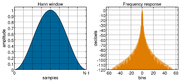
[edit] Hann window [5]

- Note that:

The Hann and Hamming windows, both of which are in the family known as "raised cosine" windows, are respectively named after Julius von Hann and Richard Hamming. The term "Hanning window" is sometimes used to refer to the Hann window.

[edit] Cosine window [5]

- also known as sine window
- cosine window describes the shape of

[edit] Lanczos window

- used in Lanczos resampling
- for the Lanczos window, sinc(x) is defined as sin(πx)/(πx)
- also known as a sinc window, because:
-
 is the main lobe of a normalized sinc function

[edit] Bartlett window (zero valued end-points)


[edit] Triangular window (non-zero end-points)


[edit] Gauss windows


[edit] Bartlett–Hann window


[edit] Blackman windows
Blackman windows are defined as:[5]


By common convention, the unqualified term Blackman window refers to α=0.16.


[edit] Kaiser windows

- Note that:

[edit] Low-resolution (high-dynamic-range) windows

[edit] Nuttall window, continuous first derivative [5]


[edit] Blackman–Harris window [5]


[edit] Blackman–Nuttall window [5]


[edit] Flat top window [5]


[edit] Other windows
| This section requires expansion. |
[edit] Bessel window
[edit] Exponential window
[edit] Tukey window
[edit] Comparison of windows
-
 Stopband attenuation of different windows
When selecting an appropriate window function for an application, this comparison graph may be useful. The most important parameter is usually the stopband attenuation close to the main lobe. However, some applications are more sensitive to the stopband attenuation far away from the cut-off frequency.
[edit] Overlapping windows
When the length of a data set to be transformed is larger than necessary to provide the desired frequency resolution, a common practice is to subdivide it into smaller sets and window them individually. To mitigate the "loss" at the edges of the window, the individual sets may overlap in time. See Welch method of power spectral analysis.
[edit] See also
[edit] Notes
- ^ Eric W. Weisstein (2003). CRC Concise Encyclopedia of Mathematics. CRC Press. ISBN 1584883472. http://books.google.com/books?id=aFDWuZZslUUC&pg=PA97&dq=apodization+function&lr=&as_brr=0&ei=27ycSPCdJZDwsgOdxIieBQ&sig=ACfU3U1EhHuuq88rRYF2W01Jj1o2Ab-6wA#PPA95,M1.
- ^ Carlo Cattani and Jeremiah Rushchitsky (2007). Wavelet and Wave Analysis As Applied to Materials With Micro Or Nanostructure. World Scientific. ISBN 9812707840. http://books.google.com/books?id=JuJKu_0KDycC&pg=PA53&dq=define+%22window+function%22+nonzero+interval&lr=&as_brr=3&ei=iyGbSKX_OJCKtAPXwaD2CQ&sig=ACfU3U1zZzq20w9GO1fbmNcvD3MlQFevsg#PPA53,M1.
- ^ Curtis Roads (2002). Microsound. MIT Press. ISBN 0262182157.
- ^ Mastering Windows: Improving Reconstruction
- ^ a b c d e f g h Windows of the form:
- ^ Loren D. Enochson and Robert K. Otnes (1968). Programming and Analysis for Digital Time Series Data. U.S. Dept. of Defense, Shock and Vibration Info. Center. pp. 142. http://books.google.com/books?id=duBQAAAAMAAJ&q=%22hamming+window%22+date:0-1970&dq=%22hamming+window%22+date:0-1970&lr=&as_brr=0&ei=4LEASfHtJoXWsgOcz7WdDA&pgis=1.

[edit] Other references
- harris, fredric j. (January 1978). ""On the use of Windows for Harmonic Analysis with the Discrete Fourier Transform"". Proceedings of the IEEE 66 (1): 51–83. Article on FFT windows which introduced many of the key metrics used to compare windows.
- Nuttall, Albert H. (February 1981). "Some Windows with Very Good Sidelobe Behavior". IEEE Transactions on Acoustics, Speech, and Signal Processing 29 (1): 84-91. Extends Harris' paper, covering all the window functions known at the time, along with key metric comparisons.
- Oppenheim, Alan V.; Schafer, Ronald W.; Buck, John A. (1999). Discrete-time signal processing. Upper Saddle River, N.J.: Prentice Hall. pp. 468–471. ISBN 0-13-754920-2.
- Bergen, S.W.A.; A. Antoniou (2004). "Design of Ultraspherical Window Functions with Prescribed Spectral Characteristics". EURASIP Journal on Applied Signal Processing 2004 (13): 2053–2065. doi:.
- Bergen, S.W.A.; A. Antoniou (2005). "Design of Nonrecursive Digital Filters Using the Ultraspherical Window Function". EURASIP Journal on Applied Signal Processing 2005 (12): 1910–1922. doi:.
- Park, Young-Seo, "System and method for generating a root raised cosine orthogonal frequency division multiplexing (RRC OFDM) modulation", US patent 7065150, published 2003, issued 2006
- LabView Help, Characteristics of Smoothing Filters, http://zone.ni.com/reference/en-XX/help/371361B-01/lvanlsconcepts/char_smoothing_windows/

