Big O notation
From Wikipedia, the free encyclopedia
In mathematics, big O notation describes the limiting behavior of a function when the argument tends towards a particular value or infinity, usually in terms of simpler functions. Big O notation allows its users to simplify functions in order to concentrate on their growth rates: different functions with the same growth rate may be represented using the same O notation.
Although developed as a part of pure mathematics, this notation is now frequently also used in computational complexity theory to describe an algorithm's usage of computational resources: the worst case or average case running time or memory usage of an algorithm is often expressed as a function of the length of its input using big O notation. This allows algorithm designers to predict the behavior of their algorithms and to determine which of multiple algorithms to use, in a way that is independent of computer architecture or clock rate. Big O notation is also used in many other fields to provide similar estimates.
Big O notation is also called Big Oh notation, Landau notation, Bachmann–Landau notation, and asymptotic notation. A description of a function in terms of big O notation usually only provides an upper bound on the growth rate of the function; associated with big O notation are several related notations, using the symbols o, Ω, ω, and Θ, to describe other kinds of bounds on asymptotic growth rates.
Contents |
[edit] Formal definition
Let f(x) and g(x) be two functions defined on some subset of the real numbers. One writes

if and only if there exists a positive real number M and a real number x0 such that

That is, for sufficiently large values of x, f(x) is upper bounded by a constant times g(x). In many contexts, the assumption that we are interested in the growth rate as the variable x goes to infinity is left unstated, and one writes more simply that f(x) = O(g(x)).
The notation can also be used to describe the behavior of f near some real number a (often, a = 0): we say

if and only if there exist positive numbers δ and M such that

If g(x) is non-zero for values of x sufficiently close to a, both of these definitions can be unified using the limit superior:
if and only if

[edit] Example
In typical usage, the formal definition of O notation is not used directly; rather, the O notation for a function f(x) is derived by the following simplification rules:
- If f(x) is a sum of several terms, the one with the largest growth rate is kept, and all others omitted.
- If f(x) is a product of several factors, any constants (terms in the product that do not depend on x) are omitted.
For example, let f(x) = 6x4 − 2x3 + 5, and suppose we wish to simplify this function, using O notation, to describe its growth rate as x approaches infinity. This function is the sum of three terms: 6x4, −2x3, and 5. Of these three terms, the one with the highest growth rate is the one with the largest exponent as a function of x, namely 6x4. Now one may apply the second rule: 6x4 is a product of 6 and x4 in which the first term does not depend on x. Omitting this term results in the simplified form x4. Thus, f(x) = O(x4).
One may confirm this calculation using the formal definition: let f(x) = 6x4 − 2x3 + 5 and g(x) = x4. Applying the formal definition from above, the statement that f(x) = O(x4) is equivalent to its expansion,
for some suitable choice of x0 and M and for all x > x0. To prove this, let x0 = 1 and M = 13. Then, for all x > x0:

so

[edit] Usage
Big O notation has two main areas of application. In mathematics, it is commonly used to describe how closely a finite series approximates a given function, especially in the case of a truncated Taylor series or asymptotic expansion. In computer science, it is useful in the analysis of algorithms. In both applications, the function g(x) appearing within the O(...) is typically chosen to be as simple as possible, omitting constant factors and lower order terms.
There are two formally close, but noticeably different, usages of this notation: infinite asymptotics and infinitesimal asymptotics. This distinction is only in application and not in principle, however—the formal definition for the "big O" is the same for both cases, only with different limits for the function argument.
[edit] Infinite asymptotics
Big O notation is useful when analyzing algorithms for efficiency. For example, the time (or the number of steps) it takes to complete a problem of size n might be found to be T(n) = 4n2 − 2n + 2.
As n grows large, the n2 term will come to dominate, so that all other terms can be neglected — for instance when n = 500, the term 4n2 is 1000 times as large as the 2n term. Ignoring the latter would have negligible effect on the expression's value for most purposes.
Further, the coefficients become irrelevant if we compare to any other order of expression, such as an expression containing a term n3 or n2. Even if T(n) = 1,000,000n2, if U(n) = n3, the latter will always exceed the former once n grows larger than 1,000,000 (T(1,000,000) = 1,000,0003= U(1,000,000)). Additionally, the number of steps depends on the details of the machine model on which the algorithm runs, but different types of machines typically vary by only a constant factor in the number of steps needed to execute an algorithm.
So the big O notation captures what remains: we write either

or

and say that the algorithm has order of n2 time complexity.
Note that "=" is not meant to express "is equal to" in its normal mathematical sense, but rather a more colloquial "is", so the second expression is technically accurate (see the "Equals sign" discussion below) while the first is a common abuse of notation.[1]
[edit] Infinitesimal asymptotics
Big O can also be used to describe the error term in an approximation to a mathematical function. For example,

expresses the fact that the error, the difference  , is smaller in absolute value than some constant times | x3 | when x is close enough to 0.
[edit] Properties
If a function f(n) can be written as a finite sum of other functions, then the fastest growing one determines the order of f(n). For example

In particular, if a function may be bounded by a polynomial in n, then as n tends to infinity, one may disregard lower-order terms of the polynomial.
O(nc) and O(cn) are very different. The latter grows much, much faster, no matter how big the constant c is (as long as it is greater than one). A function that grows faster than any power of n is called superpolynomial. One that grows more slowly than any exponential function of the form cn is called subexponential. An algorithm can require time that is both superpolynomial and subexponential; examples of this include the fastest known algorithms for integer factorization.
O(logn) is exactly the same as O(log(nc)). The logarithms differ only by a constant factor, (since log(nc) = clogn) and thus the big O notation ignores that. Similarly, logs with different constant bases are equivalent. Exponentials with different bases, on the other hand, are not of the same order. For example, 2n and 3n are not of the same order.
Changing units may or may not affect the order of the resulting algorithm. Changing units is equivalent to multiplying the appropriate variable by a constant wherever it appears. For example, if an algorithm runs in the order of n2, replacing n by cn means the algorithm runs in the order of c2n2, and the big O notation ignores the constant c2. This can be written as  . If, however, an algorithm runs in the order of 2n, replacing n with cn gives 2cn = (2c)n. This is not equivalent to 2n (unless, of course, c=1).
Changing of variable may affect the order of the resulting algorithm. For example, if an algorithm runs on the order of O(n) when n is the number of digits of the input number, then it has order O(log n) when n is the input number itself.
[edit] Product


[edit] Sum

- This implies
 , which means that O(g) is a convex cone.
- This implies
- If f and g are positive functions,
[edit] Multiplication by a constant
- Let k be a constant. Then:

[edit] Multiple variables
Big O (and little o, and Ω…) can also be used with multiple variables.
To define Big O formally for multiple variables, suppose  and
and  are two functions defined on some subset of
  . We say

if and only if

For example, the statement

asserts that there exist constants C and M such that

where g(n,m) is defined by

Note that this definition allows all of the coordinates of  to increase to infinity. In particular, the statement

(i.e.,  ) is quite different from

(i.e., 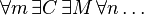 ).
).
[edit] Matters of notation
[edit] Equals sign
The statement "f(x) is O(g(x))" as defined above is usually written as f(x) = O(g(x)). This is an abuse of notation; equality of two functions is not asserted, and it cannot be since the property of being O(g(x)) is not symmetric:
 .
.
There is also a second reason why that notation is not precise. The symbol f(x) means the value of the function f for the argument x. Hence the symbol of the function is f and not f(x).
For these reasons, it would be more precise to use set notation and write  , thinking of O(g) as the set of all functions dominated by g. However, the use of the equals sign is customary. Knuth pointed out[2] (as de Bruijn[3] did) that "mathematicians customarily use the = sign as they use the word 'is' in English: Aristotle is a man, but a man isn’t necessarily Aristotle."
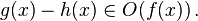
[edit] Other arithmetic operators
Big O notation can also be used in conjunction with other arithmetic operators in more complicated equations. For example, h(x) + O(f(x)) denotes the collection of functions having the growth of h(x) plus a part whose growth is limited to that of f(x). Thus,
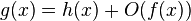
expresses the same as
[edit] Example
Suppose an algorithm is being developed to operate on a set of n elements. Its developers are interested in finding a function T(n) that will express how long the algorithm will take to run (in some arbitrary measurement of time) in terms of the number of elements in the input set. The algorithm works by first calling a subroutine to sort the elements in the set and then perform its own operations. The sort has a known time complexity of O(n2), and after the subroutine runs the algorithm must take an additional 55n3 + 2n + 10 time before it terminates. Thus the overall time complexity of the algorithm can be expressed as
- T(n) = O(n2) + 55n3 + 2n + 10
This can perhaps be most easily read by replacing O(n2) with "some function that grows asymptotically slower than n2 ". Again, this usage disregards some of the formal meaning of the "=" and "+" symbols, but it does allow one to use the big O notation as a kind of convenient placeholder.
[edit] Declaration of variables
Another feature of the notation, although less exceptional, is that function arguments may need to be inferred from the context when several variables are involved. The following two right-hand side big O notations have dramatically different meanings:

The first case states that f(m) exhibits polynomial growth, while the second, assuming m > 1, states that g(n) exhibits exponential growth. To avoid confusion, some authors use the notation

rather than the less explicit
[edit] Complex usages
In more complex usage, O(...) can appear in different places in an equation, even several times on each side. For example, the following are true for 
- (n + 1)2 = n2 + O(n)
- (n + O(n1 / 2))(n + O(logn))2 = n3 + O(n5 / 2)
- nO(1) = O(en)
The meaning of such statements is as follows: for any functions which satisfy each O(...) on the left side, there are some functions satisfying each O(...) on the right side, such that substituting all these functions into the equation makes the two sides equal. For example, the third equation above means: "For any function f(n) = O(1), there is some function g(n) = O(en) such that nf(n) = g(n)." In terms of the "set notation" above, the meaning is that the class of functions represented by the left side is a subset of the class of functions represented by the right side.
[edit] Orders of common functions
Here is a list of classes of functions that are commonly encountered when analyzing algorithms. In each case, c is a constant and n increases without bound. The slower-growing functions are listed first.
| Notation | Name | Example |
|---|---|---|
 |
constant | Determining if a number is even or odd; using a constant-size lookup table or hash table |
 |
inverse Ackermann | Amortized time per operation using a disjoint set |
 |
iterated logarithmic | The find algorithm of Hopcroft and Ullman on a disjoint set |
 |
log-logarithmic | Amortized time per operation using a bounded priority queue[4] |
 |
logarithmic | Finding an item in a sorted array with a binary search |
 |
polylogarithmic | Deciding if n is prime with the AKS primality test |
 |
fractional power | Searching in a kd-tree |
 |
linear | Finding an item in an unsorted list; adding two n-digit numbers |
 |
linearithmic, loglinear, or quasilinear | Performing a Fast Fourier transform; heapsort, or merge sort |
 |
quadratic | Multiplying two n-digit numbers by a simple algorithm; adding two n×n matrices; bubble sort, shell sort, quicksort, or insertion sort |
 |
cubic | Multiplying two n×n matrices by simple algorithm; finding the shortest path on a weighted digraph with the Floyd-Warshall algorithm; inverting a (dense) nxn matrix using LU or Cholesky decomposition |
 |
polynomial or algebraic | Tree-adjoining grammar parsing; maximum matching for bipartite graphs (grows faster than cubic if and only if c > 3) |
![L_n[\alpha,c], 0 < \alpha < 1=\,](http://upload.wikimedia.org/math/5/2/a/52acd8181ae48e5bf45c13868bce0371.png)  |
L-notation | Factoring a number using the special or general number field sieve |
 |
exponential or geometric | Finding the (exact) solution to the traveling salesman problem using dynamic programming; determining if two logical statements are equivalent using brute force |
 |
factorial or combinatorial | Solving the traveling salesman problem via brute-force search; finding the determinant with expansion by minors. The statement  is sometimes weakened to is sometimes weakened to  to derive simpler formulas for asymptotic complexity. to derive simpler formulas for asymptotic complexity. |
 |
double exponential | Deciding the truth of a given statement in Presburger arithmetic |
Remarks:
Larger growth, such as the single-valued version of the Ackermann function, A(n,n) is uncommon in practice.
For any k > 0 and c > 0, O(nc(logn)k) is a subset of O(nc + a) for any a > 0, so may be considered as a polynomial with some bigger order.
[edit] Related asymptotic notations
Big O is the most commonly used asymptotic notation for comparing functions, although in many cases Big O may be replaced with Big Theta Θ for asymptotically tighter bounds (Theta, see below). Here, we define some related notations in terms of Big O, progressing up to the family of Bachmann–Landau notations to which Big O notation belongs.
[edit] Little-o notation
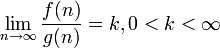
The relation  is read as "f(x) is little-o of g(x)". Intuitively, it means that g(x) grows much faster than f(x). It assumes that f and g are both functions of one variable. Formally, it states that the limit of f(x) / g(x) is zero, as x approaches infinity. For algebraically defined functions f(x) and g(x),
  is generally found using L'Hôpital's rule.
For example,


Little-o notation is common in mathematics but rarer in computer science. In computer science the variable (and function value) is most often a natural number. In math, the variable and function values are often real numbers. The following properties can be useful:

 (and thus the above properties apply with most combinations of o and O).
As with big O notation, the statement "f(x) is o(g(x))" is usually written as f(x) = o(g(x)), which is a slight abuse of notation.
[edit] The family of Bachmann–Landau notations
| Notation | Name | Intuition | As , eventually... |
Definition |
|---|---|---|---|---|
 |
Big Omicron; Big O; Big Oh | f is bounded above by g (up to constant factor) asymptotically | 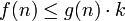 |
 or or  |
 (Older math papers sometimes this in the weaker sense that f=o(g) is false) (Older math papers sometimes this in the weaker sense that f=o(g) is false) |
Big Omega | f is bounded below by g (up to constant factor) asymptotically |  |
 |
 |
Big Theta | f is bounded both above and below by g asymptotically |  |
 |
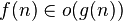 |
Small Omicron; Small O; Small Oh | f is dominated by g asymptotically |  |
 |
 |
Small Omega | f dominates g asymptotically | 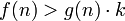 |
 |
 |
on the order of | f is equal to g asymptotically |  |
 |
Bachmann–Landau notation was designed around several mnemonics, as shown in the As , eventually... column above and in the bullets below. To conceptually access these mnemonics, "omicron" can be read "o-micron" and "omega" can be read "o-mega". Also, the lower-case versus capitalization of the Greek letters in Bachmann–Landau notation is mnemonic.
- the o-micron mnemonic: The o-micron reading of and of can be thought of as "O-smaller than" and "o-smaller than", respectively. This micro/smaller mnemonic refers to: for sufficiently large input parameter(s), f grows at a rate that may henceforth be less than cg regarding
 or
or  .
. - the o-mega mnemonic: The o-mega reading of and of can be thought of as "O-larger than". This mega/larger mnemonic refers to: for sufficiently large input parameter(s), f grows at a rate that may henceforth be greater than cg regarding
 or
or  .
. - the upper-case mnemonic: This mnemonic reminds us when to use the upper-case Greek letters in and : for sufficiently large input parameter(s), f grows at a rate that may henceforth be equal to cg regarding .
- the lower-case mnemonic: This mnemonic reminds us when to use the lower-case Greek letters in and : for sufficiently large input parameter(s), f grows at a rate that is henceforth inequal to cg regarding .
Aside from Big O notation, the Big Theta Θ and Big Omega Ω notations are the two most often used in computer science; the Small Omega ω notation is rarely used in computer science.
Informally, especially in computer science, the Big O notation often is permitted to be somewhat abused to describe an asymptotic tight bound where using Big Theta Θ notation might be more factually appropriate in a given context. For example, when considering a function T(n) = 73n3 + 22n2 + 58, all of the following are generally acceptable, but tightnesses of bound (i.e., bullets 2 and 3 below) are usually strongly preferred over laxness of bound (i.e., bullet 1 below).
- T(n) = O(n100), which is identical to
- T(n) = O(n3), which is identical to

- T(n) = Θ(n3), which is identical to

The equivalent English statements are respectively:
- T(n) grows asymptotically as fast or more slowly than n100
- T(n) grows asymptotically as fast or more slowly than n3
- T(n) grows asymptotically as fast as n3.
So while all three statements are true, progressively more information is contained in each. In some fields, however, the Big O notation (bullets number 2 in the lists above) would be used more commonly than the Big Theta notation (bullets number 3 in the lists above) because functions that grow more slowly are more desirable. For example, if T(n) represents the running time of a newly developed algorithm for input size n, the inventors and users of the algorithm might be more inclined to put an upper asymptotic bound on how long it will take to run without making an explicit statement about the lower asymptotic bound.
[edit] Extensions to the Bachmann–Landau notations
Another notation sometimes used in computer science is Õ (read soft-O).  is shorthand for f(n) = O(g(n)logkg(n)) for some k. Essentially, it is Big O notation, ignoring logarithmic factors because the growth-rate effects of some other super-logarithmic function indicate a growth-rate explosion for large-sized input parameters that is more important to predicting bad run-time performance than the finer-point effects contributed by the logarithmic-growth factor(s). This notation is often used to obviate the "nitpicking" within growth-rates that are stated as too tightly bounded for the matters at hand (since logkn is always o(nε) for any constant k and any ε > 0).
The L notation, defined as
![L_n[\alpha,c]=O\left(e^{(c+o(1))(\ln n)^\alpha(\ln\ln n)^{1-\alpha}}\right),](http://upload.wikimedia.org/math/a/7/4/a742357e75a2dd425a7ff99159b0fbe0.png)
is convenient for functions that are between polynomial and exponential.
[edit] Generalizations and related usages
The generalization to functions taking values in any normed vector space is straightforward (replacing absolute values by norms), where f and g need not take their values in the same space. A generalization to functions g taking values in any topological group is also possible.
The "limiting process" x→xo can also be generalized by introducing an arbitrary filter base, i.e. to directed nets f and g.
The o notation can be used to define derivatives and differentiability in quite general spaces, and also (asymptotical) equivalence of functions,

which is an equivalence relation and a more restrictive notion than the relationship "f is Θ(g)" from above. (It reduces to  if f and g are positive real valued functions.) For example, 2x is Θ(x), but 2x − x is not o(x).
[edit] Graph theory
It is often useful to bound the running time of graph algorithms. Unlike most other computational problems, for a graph G = (V, E) there are two relevant parameters describing the size of the input: the number |V| of vertices in the graph and the number |E| of edges in the graph. Inside asymptotic notation (and only there), it is common to use the symbols V and E, when someone really means |V| and |E|. We adopt this convention here to simplify asymptotic functions and make them easily readable. The symbols V and E are never used inside asymptotic notation with their literal meaning, so this abuse of notation does not risk ambiguity. For example O(E + VlogV) means  for a suitable metric of graphs. Another common convention—referring to the values |V| and |E| by the names n and m, respectively—sidesteps this ambiguity.
[edit] History
The notation was first introduced by number theorist Paul Bachmann in 1894, in the second volume of his book Analytische Zahlentheorie ("analytic number theory"), the first volume of which (not yet containing big O notation) was published in 1892.[5] The notation was popularized in the work of a number theorist Edmund Landau; hence it is sometimes called a Landau symbol. It was popularized in computer science by Donald Knuth, who (re)introduced the related Omega and Theta notations.[6] He also noted that the (then obscure) Omega notation had been introduced by Hardy and Littlewood[7] under a slightly different meaning, and proposed the current definition. The big-O, standing for "order of", was originally a capital omicron; today the identical-looking Latin capital letter O is used, but never the digit zero.
|
|
It has been suggested that Hardy notation be merged into this article or section. (Discuss) |
[edit] See also
| The Wikibook Data Structures has a page on the topic of |
- Asymptotic expansion: Approximation of functions generalizing Taylor's formula
- Asymptotically optimal: A phrase frequently used to describe an algorithm that has an upper bound asymptotically within a constant of a lower bound for the problem
- Hardy notation: A different asymptotic notation
- Limit superior and limit inferior: An explanation of some of the limit notation used in this article
- Nachbin's theorem: A precise method of bounding complex analytic functions so that the domain of convergence of integral transforms can be stated
- Op (statistics)
[edit] References
- ^ Thomas H. Cormen et al., 2001, Introduction to Algorithms, Second Edition
- ^ Donald Knuth (June/July 1998), "Teach Calculus with Big O", Notices of the American Mathematical Society 45 (6): 687, http://www.ams.org/notices/199806/commentary.pdf (Unabridged version)
- ^ N. G. de Bruijn (1958), Asymptotic Methods in Analysis, Amsterdam: North-Holland, p. 5, http://books.google.com/books?id=_tnwmvHmVwMC&pg=PA5&vq=%22The+trouble+is%22
- ^ Kurt Mehlhorn and Stefan Naher, "Bounded ordered dictionaries in O(log log N) time and O(n) space", Information Processing Letters (1990).
- ^ Nicholas J. Higham, Handbook of writing for the mathematical sciences, SIAM. ISBN 0898714206, p. 25
- ^ Donald Knuth. Big Omicron and big Omega and big Theta, ACM SIGACT News, Volume 8, Issue 2, 1976.
- ^ G. H. Hardy and J. E. Littlewood, Some problems of Diophantine approximation, Acta Mathematica 37 (1914), p. 225
[edit] Further reading
- Paul Bachmann. Die Analytische Zahlentheorie. Zahlentheorie. pt. 2 Leipzig: B. G. Teubner, 1894.
- Edmund Landau. Handbuch der Lehre von der Verteilung der Primzahlen. 2 vols. Leipzig: B. G. Teubner, 1909.
- G. H. Hardy. Orders of Infinity: The 'Infinitärcalcül' of Paul du Bois-Reymond, 1910.
- Marian Slodicka (Slodde vo de maten) & Sandy Van Wontergem. Mathematical Analysis I. University of Ghent, 2004.
- Donald Knuth. The Art of Computer Programming, Volume 1: Fundamental Algorithms, Third Edition. Addison-Wesley, 1997. ISBN 0-201-89683-4. Section 1.2.11: Asymptotic Representations, pp.107–123.
- Thomas H. Cormen, Charles E. Leiserson, Ronald L. Rivest, and Clifford Stein. Introduction to Algorithms, Second Edition. MIT Press and McGraw-Hill, 2001. ISBN 0-262-03293-7. Section 3.1: Asymptotic notation, pp.41–50.
- Michael Sipser (1997). Introduction to the Theory of Computation. PWS Publishing. ISBN 0-534-94728-X. Pages 226–228 of section 7.1: Measuring complexity.
- Jeremy Avigad, Kevin Donnelly. Formalizing O notation in Isabelle/HOL
- Paul E. Black, "big-O notation", in Dictionary of Algorithms and Data Structures [online], Paul E. Black, ed., U.S. National Institute of Standards and Technology. 11 March 2005. Retrieved December 16, 2006.
- Paul E. Black, "little-o notation", in Dictionary of Algorithms and Data Structures [online], Paul E. Black, ed., U.S. National Institute of Standards and Technology. 17 December 2004. Retrieved December 16, 2006.
- Paul E. Black, "Ω", in Dictionary of Algorithms and Data Structures [online], Paul E. Black, ed., U.S. National Institute of Standards and Technology. 17 December 2004. Retrieved December 16, 2006.
- Paul E. Black, "ω", in Dictionary of Algorithms and Data Structures [online], Paul E. Black, ed., U.S. National Institute of Standards and Technology. 29 November 2004. Retrieved December 16, 2006.
- Paul E. Black, "Θ", in Dictionary of Algorithms and Data Structures [online], Paul E. Black, ed., U.S. National Institute of Standards and Technology. 17 December 2004. Retrieved December 16, 2006.

