Divergence

From Wikipedia, the free encyclopedia

For other uses, see Divergence (disambiguation).

"div" redirects here. For other uses, see div (disambiguation).

In vector calculus, the divergence is an operator that measures the magnitude of a vector field's source or sink at a given point; the divergence of a vector field is a (signed) scalar. For example, for a vector field that denotes the velocity of air expanding as it is heated, the divergence of the velocity field would have a positive value because the air expands. If the air cools and contracts, the divergence is negative. In this specific example the divergence could be thought of as a measure of the change in density.

A vector field that has zero divergence everywhere is called solenoidal.

[edit] Application in Cartesian coordinates

Let x, y, z be a system of Cartesian coordinates on a 3-dimensional Euclidean space, and let i, j, k be the corresponding basis of unit vectors.

The divergence of a continuously differentiable vector field F = F_x i + F_y j + F_z k is defined to be the scalar-valued function:

$\operatorname{div}\,\mathbf{F} = \nabla\cdot\mathbf{F} =\frac{\partial F_x}{\partial x} +\frac{\partial F_y}{\partial y} +\frac{\partial F_z}{\partial z }.$

Although expressed in terms of coordinates, the result is invariant under orthogonal transformations, as the physical interpretation suggests.

The common notation for the divergence ∇·F is a convenient mnemonic, where the dot denotes an operation reminiscent of the dot product: take the components of ∇ (see del), apply them to the components of F, and sum the results. As a result, this is considered an abuse of notation.

[edit] Physical interpretation as source density

In physical terms, the divergence of a three dimensional vector field is the extent to which the vector field flow behaves like a source or a sink at a given point. It is a local measure of its "outgoingness"—the extent to which there is more exiting an infinitesimal region of space than entering it. If the divergence is nonzero at some point then there must be a source or sink at that position^[1].

An alternative but equivalent definition, gives the divergence as the derivative of the net flow of the vector field across the surface of a small sphere relative to the volume of the sphere. (Note that we are imagining the vector field to be like the velocity vector field of a fluid (in motion) when we use the terms flow, sink and so on.) Formally,

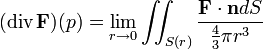
$( \operatorname{div}\,\mathbf{F}) (p) = \lim_{r \rightarrow 0} \iint_{S(r)} {\mathbf{F}\cdot\mathbf{n}dS \over \frac{4}{3} \pi r^3 }$

where S(r) denotes the sphere of radius r about a point p in R³, and the integral is a surface integral taken with respect to n, the normal to that sphere.

Instead of a sphere, any other volume $Δ V$ is possible, if instead of $\frac{4\pi r^3}{3}$ one writes $|\,\Delta V\,|\,.$ From this definition it also becomes explicitly visible that ${\rm div}\,\,{\mathbf v}$ can be seen as the source density of the flux $\mathbf v(\mathbf r)$

In light of the physical interpretation, a vector field with constant zero divergence is called incompressible – in this case, no net flow can occur across any closed surface.

The intuition that the sum of all sources minus the sum of all sinks should give the net flow outwards of a region is made precise by the divergence theorem.

[edit] Decomposition theorem

Main article: Helmholtz decomposition

It can be shown that any stationary flux $\mathbf v(\mathbf r)$ which is at least two times continuously differentiable in ${\mathbb R}^3$ and vanishes sufficiently fast for $|\mathbf r|\to \infty$ can be decomposed into an irrotational part $\mathbf E(\mathbf r)$ and a source-free part $\mathbf B(\mathbf r)\,.$ Moreover, these parts are explicitly determined by the respective source-densities (see above) and circulation densities (see the article Curl):

For the irrotational part one has

$\mathbf E=-\nabla \Phi(\mathbf r)\,,$ with $\Phi (\mathbf r)=\int_{\mathbb R^3}\,{\rm d}^3\mathbf r'\,\frac{{\rm div}\,\mathbf v(\mathbf r')}{4\pi|\mathbf r-\mathbf r'|}\,.$

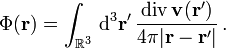
The source-free part, $\mathbf B$ , can be similarly written: one only has to replace the scalar potential $\Phi (\mathbf r)$ by a vector potential $\mathbf A(\mathbf r)$ and the terms $-\nabla \Phi$ by $+\nabla\times\mathbf A$ , and finally the source-density ${\rm div}\,\mathbf v$ by the circulation-density $\nabla \times\mathbf v\,.$

This "decomposition theorem" is in fact a by-product of the stationary case of electrodynamics. It is a special case of the more general Helmholtz decomposition which works in dimensions greater than three as well.

[edit] Properties

The following properties can all be derived from the ordinary differentiation rules of calculus. Most importantly, the divergence is a linear operator, i.e.

$\operatorname{div}( a\mathbf{F} + b\mathbf{G} ) = a\;\operatorname{div}( \mathbf{F} ) + b\;\operatorname{div}( \mathbf{G} )$

for all vector fields F and G and all real numbers a and b.

There is a product rule of the following type: if φ is a scalar valued function and F is a vector field, then

$\operatorname{div}(\varphi \mathbf{F}) = \operatorname{grad}(\varphi) \cdot \mathbf{F} + \varphi \;\operatorname{div}(\mathbf{F}),$

or in more suggestive notation

$\nabla\cdot(\varphi \mathbf{F}) = (\nabla\varphi) \cdot \mathbf{F} + \varphi \;(\nabla\cdot\mathbf{F}).$

Another product rule for the cross product of two vector fields F and G in three dimensions involves the curl and reads as follows:

$\operatorname{div}(\mathbf{F}\times\mathbf{G}) = \operatorname{curl}(\mathbf{F})\cdot\mathbf{G} \;-\; \mathbf{F} \cdot \operatorname{curl}(\mathbf{G}),$

or

$\nabla\cdot(\mathbf{F}\times\mathbf{G}) = (\nabla\times\mathbf{F})\cdot\mathbf{G} - \mathbf{F}\cdot(\nabla\times\mathbf{G}).$

The Laplacian of a scalar field is the divergence of the field's gradient.

The divergence of the curl of any vector field (in three dimensions) is constant and equal to zero. If a vector field F with zero divergence is defined on a ball in R³, then there exists some vector field G on the ball with F = curl(G). For regions in R³ more complicated than balls, this latter statement might be false (see Poincaré lemma). The degree of failure of the truth of the statement, measured by the homology of the chain complex

$\{\mbox{scalar fields on }U\} \;$

$\to\{\mbox{vector fields on }U\} \;$

$\to\{\mbox{scalar fields on }U\} \;$

(where the first map is the gradient, the second is the curl, the third is the divergence) serves as a nice quantification of the complicatedness of the underlying region U. These are the beginnings and main motivations of de Rham cohomology.

[edit] Relation with the exterior derivative

One can establish a parallel between the divergence and a particular case of the exterior derivative, when it takes a 2-form to a 3-form in R³. If we define:

$\alpha=F_1\ dy\wedge dz + F_2\ dz\wedge dx + F_3\ dx\wedge dy$

its exterior derivative $d α$ is given by

$d\alpha = \left( \frac{\partial F_1}{\partial x} +\frac{\partial F_2}{\partial y} +\frac{\partial F_3}{\partial z} \right) dx\wedge dy\wedge dz$

[edit] Generalizations

The divergence of a vector field can be defined in any number of dimensions. If

$\mathbf{F}=(F_1, F_2, \dots, F_n),$

in a Euclidean coordinate system where $\mathbf{x}=(x_1, x_2, \dots, x_n)$ and $d\mathbf{x}=(dx_1, dx_2, \dots, dx_n)$ , define

$\operatorname{div}\,\mathbf{F} = \nabla\cdot\mathbf{F} =\frac{\partial F_1}{\partial x_1} +\frac{\partial F_2}{\partial x_2}+\cdots +\frac{\partial F_n}{\partial x_n}.$

The appropriate expression is more complicated in curvilinear coordinates.

For any n, the divergence is a linear operator, and it satisfies the "product rule"

$\nabla\cdot(\varphi \mathbf{F}) = (\nabla\varphi) \cdot \mathbf{F} + \varphi \;(\nabla\cdot\mathbf{F}).$

for any scalar-valued function φ.

The divergence can be defined on any manifold of dimension n with a volume form (or density) $μ$ e.g. a Riemannian or Lorentzian manifold. Generalising the construction of a two form for a vectorfield on $\mathbb{R}^3$ , on such a manifold a vectorfield X defines a n-1 form $j = i X μ$ obtained by contracting X with $μ$ . The divergence is then the function defined by

$d j = \operatorname{div}(X) \mu$

Standard formulas for the Lie derivative allow us to reformulate this as

$\mathcal{L}_X \mu = \operatorname{div}(X) \mu$

This means that the divergence measures the rate of expansion of a volume element as we let it flow with the vectorfield.

On a Riemannian or Lorentzian manifold the divergence with respect to the metric volume form can be computed in terms of the Levi Civita connection $\nabla$

$\operatorname{div}(X) = \nabla\cdot X = X^a_{;a}$

where the second expression is the contraction of the vectorfield valued 1 -form $\nabla X$ with itself and the last expression is the traditional coordinate expression used by physicists.

[edit] See also

[edit] References

Brewer, Jess H. (1999-04-07). "DIVERGENCE of a Vector Field". Vector Calculus. http://musr.phas.ubc.ca/~jess/hr/skept/Gradient/node4.html. Retrieved on 2007-09-28.
Theresa M. Korn; Korn, Granino Arthur. Mathematical Handbook for Scientists and Engineers: Definitions, Theorems, and Formulas for Reference and Review. New York: Dover Publications. pp. 157–160. ISBN 0-486-41147-8.

^ DIVERGENCE of a Vector Field

[edit] External links

The idea of divergence and curl

[0] DIVERGENCE of a Vector Field

[1]

Divergence

From Wikipedia, the free encyclopedia

Contents

[edit] Application in Cartesian coordinates

[edit] Physical interpretation as source density

[edit] Decomposition theorem

[edit] Properties

[edit] Relation with the exterior derivative

[edit] Generalizations

[edit] See also

[edit] References

[edit] External links

Views

Personal tools

Navigation

Search

Interaction

Toolbox

Languages