Corner detection
From Wikipedia, the free encyclopedia
| Feature detection | |
 Output of a typical corner detection algorithm |
|
| Edge detection | |
|---|---|
| Canny | |
| Canny-Deriche | |
| Differential | |
| Sobel | |
| Interest point detection | |
| Corner detection | |
| Harris operator | |
| Shi and Tomasi | |
| Level curve curvature | |
| SUSAN | |
| FAST | |
| Blob detection | |
| Laplacian of Gaussian (LoG) | |
| Difference of Gaussians (DoG) | |
| Determinant of Hessian (DoH) | |
| Maximally stable extremal regions | |
| Ridge detection | |
| Affine invariant feature detection | |
| Affine shape adaptation | |
| Harris affine | |
| Hessian affine | |
| Feature description | |
| SIFT | |
| SURF | |
| GLOH | |
| LESH | |
| Scale-space | |
| Scale-space axioms | |
| Implementation details | |
| Pyramids | |
Corner detection or the more general terminology interest point detection is an approach used within computer vision systems to extract certain kinds of features and infer the contents of an image. Corner detection is frequently used in motion detection, image matching, tracking, image mosaicing, panorama stitching, 3D modelling and object recognition.
[edit] Formalization
A corner can be defined as the intersection of two edges. A corner can also be defined as a point for which there are two dominant and different edge directions in a local neighbourhood of the point. An interest point is a point in an image which has a well-defined position and can be robustly detected. This means that an interest point can be a corner but it can also be, for example, an isolated point of local intensity maximum or minimum, line endings, or a point on a curve where the curvature is locally maximal. In practice, most so-called corner detection methods detect interest points in general rather than corners in particular. As a consequence, if only corners are to be detected it is necessary to do a local analysis of detected interest points to determine which of these are real corners. Unfortunately, in the literature, "corner", "interest point" and "feature" are used somewhat interchangeably, which rather clouds the issue. Specifically, there are several blob detectors that can be referred to as "interest point operators", but which are sometimes erroneously referred to as "corner detectors". Moreover, there exists a notion of ridge detection to capture the presence of elongated objects.
Corner detectors are not usually very robust and often require expert supervision or large redundancies introduced to prevent the effect of individual errors from dominating the recognition task. The quality of a corner detector is often judged based on its ability to detect the same corner in multiple images, which are similar but not identical, for example having different lighting, translation, rotation and other transforms. A simple approach to corner detection in images is using correlation, but this gets very computationally expensive and suboptimal. An alternative approach used frequently is based on a method proposed by Harris and Stephens (below), which in turn is an improvement of a method by Moravec.
[edit] The Moravec corner detection algorithm
This is one of the earliest corner detection algorithms and defines a corner to be a point with low self-similarity. The algorithm tests each pixel in the image to see if a corner is present, by considering how similar a patch centered on the pixel is to nearby, largely overlapping patches. The similarity is measured by taking the sum of squared differences (SSD) between the two patches. A lower number indicates more similarity.
If the pixel is in a region of uniform intensity, then the nearby patches will look similar. If the pixel is on an edge, then nearby patches in a direction perpendicular to the edge will look quite different, but nearby patches in a direction parallel to the edge will result only in a small change. If the pixel is on a feature with variation in all directions, then none of the nearby patches will look similar.
The corner strength is defined as the smallest SSD between the patch and its neighbors (horizontal, vertical and on the two diagonals). If this number is locally maximal, then a feature of interest is present.
As pointed out by Moravec, one of the main problems with this operator is that it is not isotropic: if an edge is present that is not in the direction of the neighbours, then it will not be detected as an interest point.
[edit] The Harris & Stephens / Plessey corner detection algorithm
Harris and Stephens improved upon Moravec's corner detector by considering the differential of the corner score with respect to direction directly, instead of using shifted patches. It should be noted that this corner score is often referred to as autocorrelation, since the term is used in the paper in which this detector is described. However, the mathematics in the paper clearly indicate that the SSD is used.
Without loss of generality, we will assume a grayscale 2-dimensional image is used. Let this image be given by I. Consider taking an image patch over the area (u,v) and shifting it by (x,y). The weighted sum of square difference between these two patches, denoted S, is given by:

Approximating I(u + x,v + y) by Taylor expansion,

we obtain

where Ix and Iy are partial derivatives of I, or equivalently
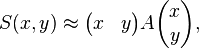
where A is the structure tensor,

is a Harris matrix and angle brackets denote averaging (summation over (u,v)). If a circular window (or circularly weighted window, such as a Gaussian) is used, then the response will be isotropic.
A corner (or in general an interest point) is characterized by a large variation of S in all directions of the vector  . By analyzing the eigenvalues of A, this characterization can be expressed in the following way: A should have two "large" eigenvalues for an interest point. Based on the magnitudes of the eigenvalues, the following inferences can be made based on this argument:
- If
 and
and  then this pixel (x,y) has no features of interest.
 - If and λ2 has some large positive value, then an edge is found.
- If λ1 and λ2 have large positive values, then a corner is found.
Harris and Stephens note that exact computation of the eigenvalues is computationally expensive, since it requires the computation of a square root, and instead suggest the following function Mc, where κ is a tunable sensitivity parameter:

Therefore, the algorithm does not have to actually compute the eigenvalue decomposition of the matrix A and instead it is sufficient to evaluate the determinant and trace of A to find corners, or rather interest points in general.
The value of κ has to be determined empirically, and in the literature values in the range 0.04 - 0.15 have been reported as feasible.
The covariance matrix for the corner position is A − 1, i.e. 
[edit] The multi-scale Harris operator
The computation of the second moment matrix (sometimes also referred to as the structure tensor) A in the Harris operator, requires the computation of image derivatives Ix,Iy in the image domain as well as the summation of non-linear combinations of these derivatives over local neighbourhoods. Since the computation of derivatives usually involves a stage of scale-space smoothing, an operational definition of the Harris operator requires two scale parameters: (i) a local scale for smoothing prior to the computation of image derivatives, and (ii) an integration scale for accumulating the non-linear operations on derivative operators into an integrated image descriptor.
With I denoting the original image brightness, let L denote the scale-space representation of I obtained by convolution with a Gaussian kernel

with local scale parameter t:

and let  and
and  denote the partial derivatives of L. Moreover, introduce a Gaussian window function g(x,y,s) with integration scale parameter s. Then, the multi-scale second-moment matrix (Lindeberg and Garding 1997) can be defined as

Then, we can compute eigenvalues of μ in a similar way as the eigenvalues of A and define the multi-scale Harris corner measure as
 .
.
Concerning the choice of the local scale parameter t and the integration scale parameter s, these scale parameters are usually coupled by a relative integration scale parameter γ such that s = γ2t, where γ is usually chosen in the interval ![[\sqrt{2}, 2]](http://upload.wikimedia.org/math/b/7/0/b70f069d9a2b137b257050f18174f544.png) . Thus, we can compute the multi-scale Harris corner measure Mc(x,y;t,γ2t) at any scale t in scale-space to obtain a multi-scale corner detector, which responds to corner structures of varying sizes in the image domain (Baumberg 2000).
. Thus, we can compute the multi-scale Harris corner measure Mc(x,y;t,γ2t) at any scale t in scale-space to obtain a multi-scale corner detector, which responds to corner structures of varying sizes in the image domain (Baumberg 2000).
In practice, this multi-scale corner detector is often complemented by a scale selection step, where the scale-normalized Laplacian operator (Lindeberg 1998)

is computed at every scale in scale-space and scale adapted corner points with automatic scale selection (the "Harris-Laplace operator") are computed from the points that are simultaneously (Mikolajczyk and Schmid 2004):
- spatial maxima of the multi-scale corner measure Mc(x,y;t,γ2t)
- local maxima or minima over scales of the scale-normalized Laplacian operator

 .
.

[edit] The Shi and Tomasi corner detection algorithm
Note that this is also sometimes referred to as the Kanade-Tomasi corner detector.
The corner detector is strongly based on the Harris corner detector. The authors show that for image patches undergoing affine transformations, min(λ1,λ2) is a better measure of corner strength than Mc.
[edit] The level curve curvature approach
An earlier approach to corner detection is to detect points where the curvature of level curves and the gradient magnitude are simultaneously high. A differential way to detect such points is to compute the rescaled level curve curvature (the product of the level curve curvature and the gradient magnitude raised to the power of three)

and to detect positive maxima and negative minima of this differential expression at some scale t in the scale-space representation L of the original image. A main problem with this approach, however, is that it is sensitive to noise and to the choice of the scale level. A better method is to compute the γ-normalized rescaled level curve curvature

with γ = 7 / 8 and to detect signed scale-space maxima of this expression, that are points and scales that are positive maxima and negative minima with respect to both space and scale

in combination with a complementary localization step to handle the increase in localization error at coarser scales (Lindeberg 1998). In this way, larger scale values will be associated with rounded corners of large spatial extent while smaller scale values will be associated with sharp corners with small spatial extent. This approach is the first corner detector with automatic scale selection (prior to the "Harris-Laplace operator" above) and has been used by (Bretzner and Lindeberg 1998) for tracking corners under large scale variations in the image domain.
[edit] LoG, DoG, and DoH feature detection
LoG is an acronym standing for Laplacian of Gaussian, DoG is an acronym standing for Difference of Gaussians (DoG is an approximation of LoG), and DoH is an acronym standing for Determinant of the Hessian.
These detectors are more completely described in blob detection, however the LoG and DoG blobs do not necessarily make highly selective features, since these operators may also respond to edges. To improve the corner detection ability of the DoG detector, the feature detector used in the SIFT system uses an additional post-processing stage, where the eigenvalues of the Hessian of the image at the detection scale are examined in a similar way as in the Harris operator. If the ratio of the eigenvalues is too high, then the local image is regarded as too edge-like, so the feature is rejected. The DoH operator on the other hand only responds when there are significant grey-level variations in two directions.
[edit] The Wang and Brady corner detection algorithm
The Wang and Brady detector considers the image to be a surface, and looks for places where there is large curvature along an image edge. In other words, the algorithm looks for places where the edge changes direction rapidly. The corner score, C, is given by:

where c determines how edge-phobic the detector is. The authors also note that smoothing (Gaussian is suggested) is required to reduce noise. In this case, the first term of C becomes the Laplacian (single-scale) blob detector.
Smoothing also causes displacement of corners, so the authors derive an expression for the displacement of a 90 degree corner, and apply this as a correction factor to the detected corners.
[edit] The SUSAN corner detector
SUSAN as an acronym standing for Smallest Univalue Segment Assimilating Nucleus.
For feature detection, SUSAN places a circular mask over the pixel to be tested (the nucleus). The region of the mask is M, and a pixel in this mask is represented by  . The nucleus is at
  . Every pixel is compared to the nucleus using the comparison function:

where t determines the radius, and the power of the exponent has been determined empirically. This function has the appearance of a smoothed top-hat or rectangular function. The area of the SUSAN is given by:

If c is the rectangular function, then n is the number of pixels in the mask which are within t of the nucleus. The response of the SUSAN operator is given by:
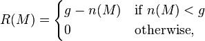
where g is named the `geometric threshold'. In other words the SUSAN operator only has a positive score if the area is small enough. The smallest USAN locally can be found using non-maximal suppression, and this is the complete SUSAN operator.
The value t determines how similar points have to be to the nucleus before they are considered to be part of the univalue segment. The value of g determines the minimum size of the univalue segment. If g is large enough, then this becomes an edge detector.
For corner detection, two further steps are used. Firstly, the centroid of the USAN if found. A proper corner will have the centroid far from the nucleus. The second step insists that all points on the line from the nucleus through the centroid out to the edge of the mask are in the SUSAN.
This technique is patented with UK patent 2272285.
[edit] The Trajkovic and Hedley corner detector
In a manner similar to SUSAN, this detector directly tests whether a patch under a pixel is self-similar by examining nearby pixels.  is the pixel to be considered, and
  is point on a circle P centered around . The point
  is the point opposite to
  along the diameter.
The response function is defined as:

This will be large when there is no direction in which the centre pixel is similar to two nearby pixels along a diameter. P is a discretised circle (a Bresenham circle), so interpolation is used for intermediate diameters to give a more isotropic response. Since any computation gives an upper bound on  , the horizontal and vertical directions are checked to see if it is worth proceeding with the complete computation of c.
[edit] The FAST feature detector
FAST is an acronym standing for Features from Accelerated Segment Test.
The feature detector considers pixels in a Bresenham circle of radius r around the candidate point. If n contiguous pixels are all brighter than the nucleus by at least t or all darker than the nucleus by t, then the pixel under the nucleus is considered to be a feature. Although r can in principle take any value, only a value of 3 is used (corresponding to a circle of 16 pixels circumference), and tests show that the best value of n is 9. This value of n is the lowest one at which edges are not detected. The resulting detector is reported{by Edward Rosten and Rohan Loveland 2008} to produce very stable features. Additionally, the ID3 algorithm is used to optimize the order in which pixels are tested, resulting in the most computationally efficient feature detector available.
Confusingly, the name of the detector is somewhat similar to the name of the paper describing Trajkovic and Hedley's detector.
[edit] Automatic synthesis of point detectors with Genetic Programming
Trujillo and Olague (2000) introduced a method by which genetic programming, one of the most advanced forms of evolutionary computation, is used to automatically synthesize image operators that can detect interest points. The terminal and function sets contain primitive operations that are common in many previously proposed man-made designs. Fitness measures the stability of each operator through the repeatability rate, and promotes a uniform dispersion of detected points across the image plane. The performance of the evolved operators has been confirmed experimentally using training and testing sequences of progressively transformed images. Hence, the proposed GP algorithm is considered to be human-competitive for the problem of interest point detection, making it one of only 60 or so results that have achieved this recognition from evolutionary computation community.
[edit] Affine-adapted interest point operators
The interest points obtained from the multi-scale Harris operator with automatic scale selection are invariant to translations, rotations and uniform rescalings in the spatial domain. The images that constitute the input to a computer vision system are, however, also subject to perspective distortions. To obtain an interest point operator that is more robust to perspective transformations, a natural approach is to devise a feature detector that is invariant to affine transformations. In practice, affine invariant interest points can be obtained by applying affine shape adaptation where the shape of the smoothing kernel is iteratively warped to match the local image structure around the interest point or equivalently a local image patch is iteratively warped while the shape of the smoothing kernel remains rotationally symmetric (Lindeberg and Garding 1997; Baumberg 2000; Mikolajczyk and Schmid 2004). Hence, besides the commonly used multi-scale Harris operator, affine shape adaptation can be applied to other corner detectors as listed in this article as well as to differential blob detectors such as the Laplacian/Difference of Gaussian operator, the determinant of the Hessian and the Hessian-Laplace operator.
[edit] References
- A. Baumberg (2000). "Reliable feature matching across widely separated views". Proceedings of IEEE Conference on Computer Vision and Pattern Recognition: pages I:1774--1781.
- L. Bretzner and T. Lindeberg (1998). "Feature tracking with automatic selection of spatial scales". Computer Vision and Image Understanding 71: pp 385--392. doi:. http://www.nada.kth.se/cvap/abstracts/cvap201.html.
- M.J. Brooks and W. Chojnacki and D. Gawley and A. van den Hengel (2001). "What Value Covariance Information in Estimating Vision Parameters?" (PDF). Proceedings of the 8th Int'l Conf. on Computer Vision 1: pp 302-308.
- K. Derpanis (2004) (PDF). The Harris Corner Detector. http://www.cse.yorku.ca/~kosta/CompVis_Notes/harris_detector.pdf.
- C. Harris and M. Stephens (1988). "A combined corner and edge detector" (PDF). Proceedings of the 4th Alvey Vision Conference: pp 147--151.
- C. Harris. (1992). "Geometry from visual motion". in A. Blake and A. Yuille. Active Vision. MIT Press, Cambridge MA.
- T. Lindeberg (1998). "Feature detection with automatic scale selection". International Journal of Computer Vision 30 (2): pp 77--116. http://www.nada.kth.se/cvap/abstracts/cvap198.html.
- T. Lindeberg and J. Garding (1997). "Shape-adapted smoothing in estimation of 3-{D} depth cues from affine distortions of local 2-{D} structure". International Journal of Computer Vision 15: pp 415--434. http://www.nada.kth.se/~tony/abstracts/LG94-ECCV.html.
- D. Lowe (2004). "Distinctive Image Features from Scale-Invariant Keypoints". International Journal of Computer Vision 60: 91. doi:. http://citeseer.ist.psu.edu/654168.html.
- K. Mikolajczyk, K. and C. Schmid (2004). "Scale and affine invariant interest point detectors" (PDF). International Journal of Computer Vision 60 (1): pp 63–86. doi:. http://www.robots.ox.ac.uk/~vgg/research/affine/det_eval_files/mikolajczyk_ijcv2004.pdf.
- H. Moravec (1980). "Obstacle Avoidance and Navigation in the Real World by a Seeing Robot Rover". Tech Report CMU-RI-TR-3 Carnegie-Mellon University, Robotics Institute. http://www.ri.cmu.edu/pubs/pub_22.html.
- E. Rosten and T. Drummond (May 2006). "Machine learning for high-speed corner detection,". European Conference on Computer Vision.
- J. Shi and C. Tomasi (June 1994). "Good Features to Track,". 9th IEEE Conference on Computer Vision and Pattern Recognition, Springer.
- S. M. Smith and J. M. Brady (May 1997). "SUSAN - a new approach to low level image processing.". International Journal of Computer Vision 23 (1): 45–78. doi:. http://citeseer.ist.psu.edu/smith95susan.html.
- S. M. Smith and J. M. Brady (January 1997), "Method for digitally processing images to determine the position of edges and/or corners therein for guidance of unmanned vehicle". UK Patent 2272285, Proprietor: Secretary of State for Defence, UK.
- C. Tomasi and T. Kanade (2004). "Detection and Tracking of Point Features". Pattern Recognition. http://www.sciencedirect.com/science?_ob=ArticleURL&_udi=B6V14-49D6WH0-1&_user=10&_rdoc=1&_fmt=&_orig=search&_sort=d&view=c&_version=1&_urlVersion=0&_userid=10&md5=cecb6ab80d45107f1cedb17aa4b211fb.
- R. Dinesh and D.S. Guru (2004). "Non-parametric adaptive region of support useful for corner detection: a novel approach". Pattern Recognition. http://www.sciencedirect.com/science?_ob=ArticleURL&_udi=B6V09-3Y450Y2-8&_coverDate=11%2F30%2F1995&_alid=442214633&_rdoc=1&_fmt=&_orig=search&_qd=1&_cdi=5641&_sort=d&view=c&_acct=C000057551&_version=1&_urlVersion=0&_userid=2493154&md5=b0979efc3df88572ec71d07e2e9f14da.
- M. Trajkovic and M. Hedley (1998). "Fast corner detection". Image and Vision Computing 16 (2): 75–87. doi:.
- Leonardo Trujillo and Gustavo Olague (2008). "Automated design of image operators that detect interest points". Evolutionary Computation 16 (4): 483–507. doi:. http://cienciascomp.cicese.mx/evovision/olague_EC_MIT.pdf.
- H. Wang and M. Brady (1995). "Real-time corner detection algorithm for motion estimation.". Image and Vision Computing 13 (9): 695–703. doi:. http://www.sciencedirect.com/science?_ob=ArticleURL&_udi=B6V09-3Y450Y2-8&_coverDate=11%2F30%2F1995&_alid=442214633&_rdoc=1&_fmt=&_orig=search&_qd=1&_cdi=5641&_sort=d&view=c&_acct=C000057551&_version=1&_urlVersion=0&_userid=2493154&md5=b0979efc3df88572ec71d07e2e9f14da.
[edit] Reference Implementations
This section provides external links to reference implementations of some of the detectors described above. These reference implementations are provided by the authors of the paper in which the detector is first described. These may contain details not present or explicit in the papers describing the features.
- DoG detection (as part of the SIFT system), Windows and x86 Linux executables
- Harris-Laplace, static Linux executables. Also contains DoG and LoG detectors and affine adaptation for all detectors included.
- FAST detector, C, C++, MATLAB source code and executables for various operating systems and architectures.
- [http://www.sciencedirect.com/science?_ob=ArticleURL&_udi=B6V14-49D6WH0-1&_user=10&_rdoc=1&_fmt=&_orig=search&_sort=d&view=c&_version=1&_urlVersion=0&_userid=10&md5=cecb6ab80d45107f1cedb17aa4b211fb
- lip-vireo,[LoG, DoG, Harris-Laplacian and Hessian-Laplacian],[SIFT, PCA-SIFT, PSIFT and Steerable Filters][Linux and Windows] executables.

