Chaos theory

From Wikipedia, the free encyclopedia

A plot of the Lorenz attractor for values r = 28, σ = 10, b = 8/3

In mathematics, chaos theory describes the behavior of certain dynamical systems – that is, systems whose states evolve with time – that may exhibit dynamics that are highly sensitive to initial conditions (popularly referred to as the butterfly effect). As a result of this sensitivity, which manifests itself as an exponential growth of perturbations in the initial conditions, the behavior of chaotic systems appears to be random. This happens even though these systems are deterministic, meaning that their future dynamics are fully defined by their initial conditions, with no random elements involved. This behavior is known as deterministic chaos, or simply chaos.

Chaotic behavior is also observed in natural systems, such as the weather. This may be explained by a chaos-theoretical analysis of a mathematical model of such a system, embodying the laws of physics that are relevant for the natural system.

[edit] Overview

Chaotic behavior has been observed in the laboratory in a variety of systems including electrical circuits, lasers, oscillating chemical reactions, fluid dynamics, and mechanical and magneto-mechanical devices. Observations of chaotic behavior in nature include the dynamics of satellites in the solar system, the time evolution of the magnetic field of celestial bodies, population growth in ecology, the dynamics of the action potentials in neurons, and molecular vibrations. Everyday examples of chaotic systems include weather and climate.^[1] There is some controversy over the existence of chaotic dynamics in plate tectonics and in economics.^[2][3][4]

Systems that exhibit mathematical chaos are deterministic and thus orderly in some sense; this technical use of the word chaos is at odds with common parlance, which suggests complete disorder. A related field of physics called quantum chaos theory studies systems that follow the laws of quantum mechanics. Recently, another field, called relativistic chaos,^[5] has emerged to describe systems that follow the laws of general relativity.

This article tries to describe limits on the degree of disorder that computers can model with simple rules that have complex results. For example, the Lorenz system pictured is chaotic, but has a clearly defined structure. Bounded chaos is a useful term for describing models of disorder.

[edit] History

Fractal fern created using chaos game. Natural forms (ferns, clouds, mountains, etc.) may be recreated through an Iterated function system (IFS).

The first discoverer of chaos was Henri Poincaré. In 1890, while studying the three-body problem, he found that there can be orbits which are nonperiodic, and yet not forever increasing nor approaching a fixed point.^[6] In 1898 Jacques Hadamard published an influential study of the chaotic motion of a free particle gliding frictionlessly on a surface of constant negative curvature.^[7] In the system studied, "Hadamard's billiards," Hadamard was able to show that all trajectories are unstable in that all particle trajectories diverge exponentially from one another, with a positive Lyapunov exponent.

Much of the earlier theory was developed almost entirely by mathematicians, under the name of ergodic theory. Later studies, also on the topic of nonlinear differential equations, were carried out by G.D. Birkhoff,^[8] A. N. Kolmogorov,^[9][10][11] M.L. Cartwright and J.E. Littlewood,^[12] and Stephen Smale.^[13] Except for Smale, these studies were all directly inspired by physics: the three-body problem in the case of Birkhoff, turbulence and astronomical problems in the case of Kolmogorov, and radio engineering in the case of Cartwright and Littlewood.^{[citation needed]} Although chaotic planetary motion had not been observed, experimentalists had encountered turbulence in fluid motion and nonperiodic oscillation in radio circuits without the benefit of a theory to explain what they were seeing.

Despite initial insights in the first half of the twentieth century, chaos theory became formalized as such only after mid-century, when it first became evident for some scientists that linear theory, the prevailing system theory at that time, simply could not explain the observed behaviour of certain experiments like that of the logistic map. What had been beforehand excluded as measure imprecision and simple "noise" was considered by chaos theories as a full component of the studied systems.

The main catalyst for the development of chaos theory was the electronic computer. Much of the mathematics of chaos theory involves the repeated iteration of simple mathematical formulas, which would be impractical to do by hand. Electronic computers made these repeated calculations practical, while figures and images made it possible to visualize these systems. One of the earliest electronic digital computers, ENIAC, was used to run simple weather forecasting models.

Turbulence in the tip vortex from an airplane wing. Studies of the critical point beyond which a system creates turbulence was important for Chaos theory, analyzed for example by the Soviet physicist Lev Landau who developed the Landau-Hopf theory of turbulence. David Ruelle and Floris Takens later predicted, against Landau, that fluid turbulence could develop through a strange attractor, a main concept of chaos theory.

An early pioneer of the theory was Edward Lorenz whose interest in chaos came about accidentally through his work on weather prediction in 1961.^[14] Lorenz was using a simple digital computer, a Royal McBee LGP-30, to run his weather simulation. He wanted to see a sequence of data again and to save time he started the simulation in the middle of its course. He was able to do this by entering a printout of the data corresponding to conditions in the middle of his simulation which he had calculated last time.

To his surprise the weather that the machine began to predict was completely different from the weather calculated before. Lorenz tracked this down to the computer printout. The computer worked with 6-digit precision, but the printout rounded variables off to a 3-digit number, so a value like 0.506127 was printed as 0.506. This difference is tiny and the consensus at the time would have been that it should have had practically no effect. However Lorenz had discovered that small changes in initial conditions produced large changes in the long-term outcome.^[15] Lorenz's discovery, which gave its name to Lorenz attractors, proved that meteorology could not reasonably predict weather beyond a weekly period (at most).

The year before, Benoît Mandelbrot found recurring patterns at every scale in data on cotton prices.^[16] Beforehand, he had studied information theory and concluded noise was patterned like a Cantor set: on any scale the proportion of noise-containing periods to error-free periods was a constant – thus errors were inevitable and must be planned for by incorporating redundancy.^[17] Mandelbrot described both the "Noah effect" (in which sudden discontinuous changes can occur, e.g., in a stock's prices after bad news, thus challenging normal distribution theory in statistics, aka Bell Curve) and the "Joseph effect" (in which persistence of a value can occur for a while, yet suddenly change afterwards).^[18][19] In 1967, he published "How long is the coast of Britain? Statistical self-similarity and fractional dimension," showing that a coastline's length varies with the scale of the measuring instrument, resembles itself at all scales, and is infinite in length for an infinitesimally small measuring device.^[20] Arguing that a ball of twine appears to be a point when viewed from far away (0-dimensional), a ball when viewed from fairly near (3-dimensional), or a curved strand (1-dimensional), he argued that the dimensions of an object are relative to the observer and may be fractional. An object whose irregularity is constant over different scales ("self-similarity") is a fractal (for example, the Koch curve or "snowflake", which is infinitely long yet encloses a finite space and has fractal dimension equal to circa 1.2619, the Menger sponge and the Sierpiński gasket). In 1975 Mandelbrot published The Fractal Geometry of Nature, which became a classic of chaos theory. Biological systems such as the branching of the circulatory and bronchial systems proved to fit a fractal model.

Chaos was observed by a number of experimenters before it was recognized; e.g., in 1927 by van der Pol^[21] and in 1958 by R.L. Ives.^[22][23] However, Yoshisuke Ueda seems to have been the first experimenter to have identified a chaotic phenomenon as such by using an analog computer on November 27, 1961. The chaos exhibited by an analog computer is a real^[vague] phenomenon, in contrast with those that digital computers calculate, which has a different kind of limit on precision. Ueda's supervising professor, Hayashi, did not believe in chaos, and thus he prohibited Ueda from publishing his findings until 1970.^[24]

In December 1977 the New York Academy of Sciences organized the first symposium on Chaos, attended by David Ruelle, Robert May, James Yorke (coiner of the term "chaos" as used in mathematics), Robert Shaw (a physicist, part of the Eudaemons group with J. Doyne Farmer and Norman Packard who tried to find a mathematical method to beat roulette, and then created with them the Dynamical Systems Collective in Santa Cruz, California), and the meteorologist Edward Lorenz.

The following year, Mitchell Feigenbaum published the noted article "Quantitative Universality for a Class of Nonlinear Transformations", where he described logistic maps.^[25] Feigenbaum had applied fractal geometry to the study of natural forms such as coastlines. Feigenbaum notably discovered the universality in chaos, permitting an application of chaos theory to many different phenomena.

In 1979, Albert J. Libchaber, during a symposium organized in Aspen by Pierre Hohenberg, presented his experimental observation of the bifurcation cascade that leads to chaos and turbulence in convective Rayleigh–Benard systems. He was awarded the Wolf Prize in Physics in 1986 along with Mitchell J. Feigenbaum "for his brilliant experimental demonstration of the transition to turbulence and chaos in dynamical systems".^[26]

Then in 1986 the New York Academy of Sciences co-organized with the National Institute of Mental Health and the Office of Naval Research the first important conference on Chaos in biology and medicine. Bernardo Huberman thereby presented a mathematical model of the eye tracking disorder among schizophrenics.^[27] Chaos theory thereafter renewed physiology in the 1980s, for example in the study of pathological cardiac cycles.

In 1987, Per Bak, Chao Tang and Kurt Wiesenfeld published a paper in Physical Review Letters^[28] describing for the first time self-organized criticality (SOC), considered to be one of the mechanisms by which complexity arises in nature. Alongside largely lab-based approaches such as the Bak–Tang–Wiesenfeld sandpile, many other investigations have centered around large-scale natural or social systems that are known (or suspected) to display scale-invariant behaviour. Although these approaches were not always welcomed (at least initially) by specialists in the subjects examined, SOC has nevertheless become established as a strong candidate for explaining a number of natural phenomena, including: earthquakes (which, long before SOC was discovered, were known as a source of scale-invariant behaviour such as the Gutenberg–Richter law describing the statistical distribution of earthquake sizes, and the Omori law^[29] describing the frequency of aftershocks); solar flares; fluctuations in economic systems such as financial markets (references to SOC are common in econophysics); landscape formation; forest fires; landslides; epidemics; and biological evolution (where SOC has been invoked, for example, as the dynamical mechanism behind the theory of "punctuated equilibria" put forward by Niles Eldredge and Stephen Jay Gould). Worryingly, given the implications of a scale-free distribution of event sizes, some researchers have suggested that another phenomenon that should be considered an example of SOC is the occurrence of wars. These "applied" investigations of SOC have included both attempts at modelling (either developing new models or adapting existing ones to the specifics of a given natural system), and extensive data analysis to determine the existence and/or characteristics of natural scaling laws.

The same year, James Gleick published Chaos: Making a New Science, which became a best-seller and introduced general principles of chaos theory as well as its history to the broad public. At first the domains of work of a few, isolated individuals, chaos theory progressively emerged as a transdisciplinary and institutional discipline, mainly under the name of nonlinear systems analysis. Alluding to Thomas Kuhn's concept of a paradigm shift exposed in The Structure of Scientific Revolutions (1962), many "chaologists" (as some self-nominated themselves) claimed that this new theory was an example of such as shift, a thesis upheld by J. Gleick.

The availability of cheaper, more powerful computers broadens the applicability of chaos theory. Currently, chaos theory continues to be a very active area of research, involving many different disciplines (mathematics, topology, physics, population biology, biology, meteorology, astrophysics, information theory, etc.).

[edit] Chaotic dynamics

For a dynamical system to be classified as chaotic, it must have the following properties:^[30]

Assign z to z² minus the conjugate of z, plus the original value of the pixel for each pixel, then count how many cycles it took when the absolute value of z exceeds two; inversion (borders are inner set), so that you can see that it threatens to fail that third condition, even if it meets condition two.

1. it must be sensitive to initial conditions,
2. it must be topologically mixing, and
3. its periodic orbits must be dense.

Sensitivity to initial conditions means that each point in such a system is arbitrarily closely approximated by other points with significantly different future trajectories. Thus, an arbitrarily small perturbation of the current trajectory may lead to significantly different future behaviour. However, it has been shown that the first two conditions in fact imply this one.^[31]

Sensitivity to initial conditions is popularly known as the "butterfly effect," so called because of the title of a paper given by Edward Lorenz in 1972 to the American Association for the Advancement of Science in Washington, D.C. entitled Predictability: Does the Flap of a Butterfly’s Wings in Brazil set off a Tornado in Texas? The flapping wing represents a small change in the initial condition of the system, which causes a chain of events leading to large-scale phenomena. Had the butterfly not flapped its wings, the trajectory of the system might have been vastly different.

This article or section may be written in a style that is too abstract to be readily understandable by general audiences. Please improve it by defining jargon or buzzwords, and by adding examples.

Sensitivity to initial conditions is often confused with chaos in popular accounts. It can also be a subtle property, since it depends on a choice of metric, or the notion of distance in the phase space of the system. For example, consider the simple dynamical system produced by repeatedly doubling an initial value. This system has sensitive dependence on initial conditions everywhere, since any pair of nearby points will eventually become widely separated. However, it has extremely simple behaviour, as all points except 0 tend to infinity. If instead we use the bounded metric on the line obtained by adding the point at infinity and viewing the result as a circle, the system no longer is sensitive to initial conditions. For this reason, in defining chaos, attention is normally restricted to systems with bounded metrics, or closed, bounded invariant subsets of unbounded systems.^{[citation needed]}

Even for bounded systems, sensitivity to initial conditions is not identical with chaos. For example, consider the two-dimensional torus described by a pair of angles (x,y), each ranging between zero and 2π. Define a mapping that takes any point (x,y) to (2x, y + a), where a is any number such that a/2π is irrational. Because of the doubling in the first coordinate, the mapping exhibits sensitive dependence on initial conditions. However, because of the irrational rotation in the second coordinate, there are no periodic orbits, and hence the mapping is not chaotic according to the definition above.

Topologically mixing means that the system will evolve over time so that any given region or open set of its phase space will eventually overlap with any other given region. Here, "mixing" is really meant to correspond to the standard intuition: the mixing of colored dyes or fluids is an example of a chaotic system.

Linear systems are never chaotic; for a dynamical system to display chaotic behaviour it has to be nonlinear. Also, by the Poincaré–Bendixson theorem, a continuous dynamical system on the plane cannot be chaotic; among continuous systems only those whose phase space is non-planar (having dimension at least three, or with a non-Euclidean geometry) can exhibit chaotic behaviour. However, a discrete dynamical system (such as the logistic map) can exhibit chaotic behaviour in a one-dimensional or two-dimensional phase space.

[edit] Attractors

Some dynamical systems are chaotic everywhere (see e.g. Anosov diffeomorphisms) but in many cases chaotic behaviour is found only in a subset of phase space. The cases of most interest arise when the chaotic behaviour takes place on an attractor, since then a large set of initial conditions will lead to orbits that converge to this chaotic region.

An easy way to visualize a chaotic attractor is to start with a point in the basin of attraction of the attractor, and then simply plot its subsequent orbit. Because of the topological transitivity condition, this is likely to produce a picture of the entire final attractor.

Phase diagram for a damped driven pendulum, with double period motion

For instance, in a system describing a pendulum, the phase space might be two-dimensional, consisting of information about position and velocity. One might plot the position of a pendulum against its velocity. A pendulum at rest will be plotted as a point, and one in periodic motion will be plotted as a simple closed curve. When such a plot forms a closed curve, the curve is called an orbit. Our pendulum has an infinite number of such orbits, forming a pencil of nested ellipses about the origin.

[edit] Strange attractors

While most of the motion types mentioned above give rise to very simple attractors, such as points and circle-like curves called limit cycles, chaotic motion gives rise to what are known as strange attractors, attractors that can have great detail and complexity. For instance, a simple three-dimensional model of the Lorenz weather system gives rise to the famous Lorenz attractor. The Lorenz attractor is perhaps one of the best-known chaotic system diagrams, probably because not only was it one of the first, but it is one of the most complex and as such gives rise to a very interesting pattern which looks like the wings of a butterfly. Another such attractor is the Rössler map, which experiences period-two doubling route to chaos, like the logistic map.

Strange attractors occur in both continuous dynamical systems (such as the Lorenz system) and in some discrete systems (such as the Hénon map). Other discrete dynamical systems have a repelling structure called a Julia set which forms at the boundary between basins of attraction of fixed points - Julia sets can be thought of as strange repellers. Both strange attractors and Julia sets typically have a fractal structure.

The Poincaré-Bendixson theorem shows that a strange attractor can only arise in a continuous dynamical system if it has three or more dimensions. However, no such restriction applies to discrete systems, which can exhibit strange attractors in two or even one dimensional systems.

The initial conditions of three or more bodies interacting through gravitational attraction (see the n-body problem) can be arranged to produce chaotic motion.

[edit] Minimum complexity of a chaotic system

Bifurcation diagram of a logistic map, displaying chaotic behaviour past a threshold

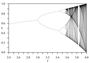
Simple systems can also produce chaos without relying on differential equations. An example is the logistic map, which is a difference equation (recurrence relation) that describes population growth over time. Another example is the Ricker model of population dynamics.

Even the evolution of simple discrete systems, such as cellular automata, can heavily depend on initial conditions. Stephen Wolfram has investigated a cellular automaton with this property, termed by him rule 30.

A minimal model for conservative (reversible) chaotic behavior is provided by Arnold's cat map.

[edit] Mathematical theory

Sharkovskii's theorem is the basis of the Li and Yorke (1975) proof that any one-dimensional system which exhibits a regular cycle of period three will also display regular cycles of every other length as well as completely chaotic orbits.

Mathematicians have devised many additional ways to make quantitative statements about chaotic systems. These include: fractal dimension of the attractor, Lyapunov exponents, recurrence plots, Poincaré maps, bifurcation diagrams, and transfer operator.

[edit] Distinguishing random from chaotic data

It can be difficult to tell from data whether a physical or other observed process is random or chaotic, because in practice no time series consists of pure 'signal.' There will always be some form of corrupting noise, even if it is present as round-off or truncation error. Thus any real time series, even if mostly deterministic, will contain some randomness.^[32]

All methods for distinguishing deterministic and stochastic processes rely on the fact that a deterministic system always evolves in the same way from a given starting point.^[32][33] Thus, given a time series to test for determinism, one can:

1. pick a test state;
2. search the time series for a similar or 'nearby' state; and
3. compare their respective time evolutions.

Define the error as the difference between the time evolution of the 'test' state and the time evolution of the nearby state. A deterministic system will have an error that either remains small (stable, regular solution) or increases exponentially with time (chaos). A stochastic system will have a randomly distributed error.^[34]

Essentially all measures of determinism taken from time series rely upon finding the closest states to a given 'test' state (i.e., correlation dimension, Lyapunov exponents, etc.). To define the state of a system one typically relies on phase space embedding methods.^[35] Typically one chooses an embedding dimension, and investigates the propagation of the error between two nearby states. If the error looks random, one increases the dimension. If you can increase the dimension to obtain a deterministic looking error, then you are done. Though it may sound simple it is not really. One complication is that as the dimension increases the search for a nearby state requires a lot more computation time and a lot of data (the amount of data required increases exponentially with embedding dimension) to find a suitably close candidate. If the embedding dimension (number of measures per state) is chosen too small (less than the 'true' value) deterministic data can appear to be random but in theory there is no problem choosing the dimension too large – the method will work.

When a non-linear deterministic system is attended by external fluctuations, its trajectories present serious and permanent distortions. Furthermore, the noise is amplified due to the inherent non-linearity and reveals totally new dynamical properties. Statistical tests attempting to separate noise from the deterministic skeleton or inversely isolate the deterministic part risk failure. Things become worse when the deterministic component is a non-linear feedback system.^[36] In presence of interactions between nonlinear deterministic components and noise the resulting nonlinear series can display dynamics that traditional tests for nonlinearity are sometimes not able to capture.^[37]

[edit] Applications

Chaos theory is applied in many scientific disciplines: mathematics, biology, computer science, economics,^[38][39][40] engineering, finance,^[41][42] philosophy, physics, politics, population dynamics, psychology, and robotics.^[43]

One of the most successful applications of chaos theory has been in ecology, where dynamical systems such as the Ricker model have been used to show how population growth under density dependence can lead to chaotic dynamics.

Chaos theory is also currently being applied to medical studies of epilepsy, specifically to the prediction of seemingly random seizures by observing initial conditions.^[44]

[edit] See also

Systems science portal

Mathematics portal

[edit] References

[edit] Scientific literature

[edit] Articles

• Li, T. Y. and Yorke, J. A. "Period Three Implies Chaos." American Mathematical Monthly 82, 985–92, 1975.
• Kolyada, S. F. "Li-Yorke sensitivity and other concepts of chaos", Ukrainian Math. J. 56 (2004), 1242–1257.
• C.E. Shannon, "A Mathematical Theory of Communication", Bell System Technical Journal, vol. 27, pp. 379–423, 623–656, July, October, 1948

[edit] Textbooks

• Alligood, K. T. (1997). Chaos: an introduction to dynamical systems. Springer-Verlag New York, LLC. ISBN 0-387-94677-2. 
• Baker, G. L. (1996). Chaos, Scattering and Statistical Mechanics. Cambridge University Press. ISBN 0-521-39511-9. 
• Badii, R.; Politi A. (1997). "Complexity: hierarchical structures and scaling in physics". Cambridge University Press. ISBN 0521663857. http://www.cambridge.org/catalogue/catalogue.asp?isbn=0521663857. 
• Devaney, Robert L. (2003). An Introduction to Chaotic Dynamical Systems, 2nd ed,. Westview Press. ISBN 0-8133-4085-3. 
• Gollub, J. P.; Baker, G. L. (1996). Chaotic dynamics. Cambridge University Press. ISBN 0-521-47685-2. 
• Gutzwiller, Martin (1990). Chaos in Classical and Quantum Mechanics. Springer-Verlag New York, LLC. ISBN 0-387-97173-4. 
• Hoover, William Graham (1999,2001). Time Reversibility, Computer Simulation, and Chaos. World Scientific. ISBN 981-02-4073-2. 
• Kiel, L. Douglas; Elliott, Euel W. (1997). Chaos Theory in the Social Sciences. Perseus Publishing. ISBN 0-472-08472-0. 
• Moon, Francis (1990). Chaotic and Fractal Dynamics. Springer-Verlag New York, LLC. ISBN 0-471-54571-6. 
• Ott, Edward (2002). Chaos in Dynamical Systems. Cambridge University Press New, York. ISBN 0-521-01084-5. 
• Strogatz, Steven (2000). Nonlinear Dynamics and Chaos. Perseus Publishing. ISBN 0-7382-0453-6. 
• Sprott, Julien Clinton (2003). Chaos and Time-Series Analysis. Oxford University Press. ISBN 0-19-850840-9. 
• Tél, Tamás; Gruiz, Márton (2006). Chaotic dynamics: An introduction based on classical mechanics. Cambridge University Press. ISBN 0-521-83912-2. 
• Tufillaro, Abbott, Reilly (1992). An experimental approach to nonlinear dynamics and chaos. Addison-Wesley New York. ISBN 0-201-55441-0. 
• Zaslavsky, George M. (2005). Hamiltonian Chaos and Fractional Dynamics. Oxford University Press. ISBN 0-198-52604-0. 

[edit] Semitechnical and popular works

• Ralph H. Abraham and Yoshisuke Ueda (Ed.), The Chaos Avant-Garde: Memoirs of the Early Days of Chaos Theory, World Scientific Publishing Company, 2001, 232 pp.
• Michael Barnsley, Fractals Everywhere, Academic Press 1988, 394 pp.
• Richard J Bird, Chaos and Life: Complexity and Order in Evolution and Thought, Columbia University Press 2003, 352 pp.
• John Briggs and David Peat, Turbulent Mirror: : An Illustrated Guide to Chaos Theory and the Science of Wholeness, Harper Perennial 1990, 224 pp.
• John Briggs and David Peat, Seven Life Lessons of Chaos: Spiritual Wisdom from the Science of Change, Harper Perennial 2000, 224 pp.
• Lawrence A. Cunningham, From Random Walks to Chaotic Crashes: The Linear Genealogy of the Efficient Capital Market Hypothesis, George Washington Law Review, Vol. 62, 1994, 546 pp.
• Leon Glass and Michael C. Mackey, From Clocks to Chaos: The Rhythms of Life, Princeton University Press 1988, 272 pp.
• James Gleick, Chaos: Making a New Science, New York: Penguin, 1988. 368 pp.
• John Gribbin, Deep Simplicity,
• L Douglas Kiel, Euel W Elliott (ed.), Chaos Theory in the Social Sciences: Foundations and Applications, University of Michigan Press, 1997, 360 pp.
• Arvind Kumar, Chaos, Fractals and Self-Organisation ; New Perspectives on Complexity in Nature , National Book Trust, 2003.
• Hans Lauwerier, Fractals, Princeton University Press, 1991.
• Edward Lorenz, The Essence of Chaos, University of Washington Press, 1996.
• Chapter 5 of Alan Marshall (2002) The Unity of nature, Imperial College Press: London
• Heinz-Otto Peitgen and Dietmar Saupe (Eds.), The Science of Fractal Images, Springer 1988, 312 pp.
• Clifford A. Pickover, Computers, Pattern, Chaos, and Beauty: Graphics from an Unseen World , St Martins Pr 1991.
• Ilya Prigogine and Isabelle Stengers, Order Out of Chaos, Bantam 1984.
• H.-O. Peitgen and P.H. Richter, The Beauty of Fractals : Images of Complex Dynamical Systems, Springer 1986, 211 pp.
• David Ruelle, Chance and Chaos, Princeton University Press 1993.
• Ivars Peterson, Newton's Clock: Chaos in the Solar System, Freeman, 1993.
• David Ruelle, Chaotic Evolution and Strange Attractors, Cambridge University Press, 1989.
• Peter Smith, Explaining Chaos, Cambridge University Press, 1998.
• Ian Stewart, Does God Play Dice?: The Mathematics of Chaos , Blackwell Publishers, 1990.
• Steven Strogatz, Sync: The emerging science of spontaneous order, Hyperion, 2003.
• Yoshisuke Ueda, The Road To Chaos, Aerial Pr, 1993.
• M. Mitchell Waldrop, Complexity : The Emerging Science at the Edge of Order and Chaos, Simon & Schuster, 1992.

[edit] External links

Wikimedia Commons has media related to: Chaos theory

• Nonlinear Dynamics Research Group with Animations in Flash
• The Chaos group at the University of Maryland
• The Chaos Hypertextbook. An introductory primer on chaos and fractals.
• Society for Chaos Theory in Psychology & Life Sciences
• Interactive live chaotic pendulum experiment, allows users to interact and sample data from a real working damped driven chaotic pendulum
• Nonlinear dynamics: how science comprehends chaos, talk presented by Sunny Auyang, 1998.
• Nonlinear Dynamics. Models of bifurcation and chaos by Elmer G. Wiens
• Gleick's Chaos (excerpt)
• Systems Analysis, Modelling and Prediction Group at the University of Oxford.
• A page about the Mackey-Glass equation.