Cauchy distribution
From Wikipedia, the free encyclopedia
Probability density function The green line is the standard Cauchy distribution |
|
Cumulative distribution function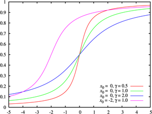 Colors match the pdf above |
|
| Parameters |  location (real) location (real) scale (real) scale (real) |
|---|---|
| Support |  |
| Probability density function (pdf) | ![\frac{1}{\pi\gamma\,\left[1 + \left(\frac{x-x_0}{\gamma}\right)^2\right]} \!](http://upload.wikimedia.org/math/1/1/0/110abf1f3bbdd637b6ddd41296caa067.png) |
| Cumulative distribution function (cdf) | 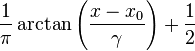 |
| Mean | not defined |
| Median | x0 |
| Mode | x0 |
| Variance | not defined |
| Skewness | not defined |
| Excess kurtosis | not defined |
| Entropy |  |
| Moment-generating function (mgf) | not defined |
| Characteristic function |  |
The Cauchy–Lorentz distribution, named after Augustin Cauchy and Hendrik Lorentz, is a continuous probability distribution. As a probability distribution, it is known as the Cauchy distribution, while among physicists, it is known as a Lorentz distribution, or a Lorentz(ian) function or the Breit–Wigner distribution.
Its importance in physics is due to it being the solution to the differential equation describing forced resonance. In spectroscopy, it is the description of the line shape of spectral lines which are subject to homogeneous broadening in which all atoms interact in the same way with the frequency range contained in the lineshape. Many mechanisms cause homogeneous broadening, most notably collision broadening.
Contents |
[edit] Characterization
[edit] Probability density function
The Cauchy distribution has the probability density function (pdf)
![\begin{align}
f(x; x_0,\gamma)&= \frac{1}{\pi\gamma \left[1 + \left(\frac{x-x_0}{\gamma}\right)^2\right]} \\[0.5em]
&= { 1 \over \pi } \left[ { \gamma \over (x - x_0)^2 + \gamma^2 } \right]
\end{align}](http://upload.wikimedia.org/math/c/9/6/c963d5240e57e4b0a2f14e7c93b9a223.png)
where x0 is the location parameter, specifying the location of the peak of the distribution, and γ is the scale parameter which specifies the half-width at half-maximum (HWHM). The amplitude of the above Lorentzian function is given by

In physics, a three-parameter Lorentzian function is often used, as follows:
![\begin{align}
f(x; x_0,\gamma,I) &= \frac{I}{\left[1 + \left(\frac{x-x_0}{\gamma}\right)^2\right]} \\[0.5em]
&= { I }\left[ { \gamma^2 \over (x - x_0)^2 + \gamma^2 } \right]
\end{align}](http://upload.wikimedia.org/math/f/b/4/fb47fd14b6002cf097d3d99a9c49469e.png)
where I is the height of the peak. The special case when x0 = 0 and γ = 1 is called the standard Cauchy distribution with the probability density function

[edit] Cumulative distribution function
The cumulative distribution function (cdf) is:

and the inverse cumulative distribution function of the Cauchy distribution is
![F^{-1}(p; x_0,\gamma) = x_0 + \gamma\,\tan\left[\pi\,\left(p-\tfrac{1}{2}\right)\right].](http://upload.wikimedia.org/math/c/5/b/c5b4a1412d33021a4bdff66d7beaa79f.png)
[edit] Properties
The Cauchy distribution is an example of a distribution which has no mean, variance or higher moments defined. Its mode and median are well defined and are both equal to x0.
When U and V are two independent normally distributed random variables with expected value 0 and variance 1, then the ratio U/V has the standard Cauchy distribution.
If X1, …, Xn are independent and identically distributed random variables, each with a standard Cauchy distribution, then the sample mean (X1 + … + Xn)/n has the same standard Cauchy distribution (the sample median, which is not affected by extreme values, can be used as a measure of central tendency). To see that this is true, compute the characteristic function of the sample mean:

where  is the sample mean. This example serves to show that the hypothesis of finite variance in the central limit theorem cannot be dropped. It is also an example of a more generalized version of the central limit theorem that is characteristic of all Lévy skew alpha-stable distributions, of which the Cauchy distribution is a special case.
The Cauchy distribution is an infinitely divisible probability distribution. It is also a strictly stable distribution.
The standard Cauchy distribution coincides with the Student's t-distribution with one degree of freedom.
The location-scale family to which the Cauchy distribution belongs is closed under linear fractional transformations with real coefficients. In this connection, see also McCullagh's parametrization of the Cauchy distributions.
[edit] Characteristic function
Let X denote a Cauchy distributed random variable. The characteristic function of the Cauchy distribution is given by

[edit] Why the mean of the Cauchy distribution is undefined
If a probability distribution has a density function f(x) then the mean is

The question is now whether this is the same thing as
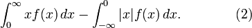
If at most one of the two terms in (2) is infinite, then (1) is the same as (2). But in the case of the Cauchy distribution, both the positive and negative terms of (2) are infinite. This means (2) is undefined. Moreover, if (1) is construed as a Lebesgue integral, then (1) is also undefined, since (1) is then defined simply as the difference (2) between positive and negative parts.
However, if (1) is construed as an improper integral rather than a Lebesgue integral, then (2) is undefined, and (1) is not necessarily well-defined. We may take (1) to mean

and this is its Cauchy principal value, which is zero, but we could also take (1) to mean, for example,

which is not zero, as can be seen easily by computing the integral.
Various results in probability theory about expected values, such as the strong law of large numbers, will not work in such cases.
[edit] Why the second moment of the Cauchy distribution is infinite
Without a defined mean, it is impossible to consider the variance or standard deviation of a standard Cauchy distribution, as these are defined with respect to the mean. But the second moment about zero can be considered. It turns out to be infinite:

[edit] Related distributions
- The ratio of two independent standard normal random variables is a standard Cauchy variable, a Cauchy(0,1). Thus the Cauchy distribution is a ratio distribution.
- The standard Cauchy(0,1) distribution arises as a special case of Student's t distribution with one degree of freedom.
- Relation to Lévy skew alpha-stable distribution:

[edit] Relativistic Breit-Wigner distribution
In nuclear and particle physics, the energy profile of a resonance is described by the relativistic Breit-Wigner distribution, while the Cauchy distribution is the (non-relativistic) Breit–Wigner distribution.

