Student's t-test

From Wikipedia, the free encyclopedia

A t-test is any statistical hypothesis test in which the test statistic has a Student's t distribution if the null hypothesis is true. It is applied when the population is assumed to be normally distributed but the sample sizes are small enough that the statistic on which inference is based is not normally distributed because it relies on an uncertain estimate of standard deviation rather than on a precisely known value.

[edit] History

The t statistic was introduced in 1908 by William Sealy Gosset, a statistician working for the Guinness brewery in Dublin, Ireland ("Student" was his pen name).^[1]^[2] Gosset had been hired due to Claude Guinness's innovative policy of recruiting the best graduates from Oxford and Cambridge to apply biochemistry and statistics to Guinness' industrial processes.^[2] Gosset devised the t-test as a way to cheaply monitor the quality of stout. He published the test in Biometrika in 1908, but was forced to use a pen name by his employer, who regarded the fact that they were using statistics as a trade secret. In fact, Gosset's identity was known to fellow statisticians.^[3]

Today, the t-test is more generally applied to the confidence that can be placed in judgments made from small samples.

[edit] Uses

Among the most frequently used t tests are:

A test of whether the mean of a normally distributed population has a value specified in a null hypothesis.
A test of the null hypothesis that the means of two normally distributed populations are equal. Given two data sets, each characterized by its mean, standard deviation and number of data points, we can use some kind of t test to determine whether the means are distinct, provided that the underlying distributions can be assumed to be normal. All such tests are usually called Student's t tests, though strictly speaking that name should only be used if the variances of the two populations are also assumed to be equal; the form of the test used when this assumption is dropped is sometimes called Welch's t test. There are different versions of the t test depending on whether the two samples are
- unpaired, independent of each other (e.g., individuals randomly assigned into two groups, measured after an intervention and compared with the other group^[4]), or
- paired, so that each member of one sample has a unique relationship with a particular member of the other sample (e.g., the same people measured before and after an intervention^[4]).

If the calculated p-value is below the threshold chosen for statistical significance (usually the 0.10, the 0.05, or 0.01 level), then the null hypothesis which usually states that the two groups do not differ is rejected in favor of an alternative hypothesis, which typically states that the groups do differ.

A test of whether the slope of a regression line differs significantly from 0.

Once a t value is determined, a p-value can be found using a table of values from Student's t-distribution.

[edit] Assumptions

Normal distribution of data (which can be tested by using a normality test, such as the Shapiro-Wilk and Kolmogorov-Smirnov tests).
Equality of variances (which can be tested by using the F test, the more robust Levene's test, Bartlett's test, or the Brown-Forsythe test).
Samples may be independent or dependent, depending on the hypothesis and the type of samples:
- Independent samples are usually two randomly selected groups
- Dependent samples are either two groups matched on some variable (for example, age) or are the same people being tested twice (called repeated measures)

Since all calculations are done subject to the null hypothesis, it may be very difficult to come up with a reasonable null hypothesis that accounts for equal means in the presence of unequal variances. In the usual case, the null hypothesis is that the different treatments have no effect — this makes unequal variances untenable. In this case, one should forgo the ease of using this variant afforded by the statistical packages. See also Behrens–Fisher problem.

One scenario in which it would be plausible to have equal means but unequal variances is when the 'samples' represent repeated measurements of a single quantity, taken using two different methods. If systematic error is negligible (e.g. due to appropriate calibration) the effective population means for the two measurement methods are equal, but they may still have different levels of precision and hence different variances.

[edit] Determining type

For novices, the most difficult issue is often whether the samples are independent or dependent. Independent samples typically consist of two groups with no relationship. Dependent samples typically consist of a matched sample (or a "paired" sample) or one group that has been tested twice (repeated measures).

Dependent t-tests are also used for matched-paired samples, where two groups are matched on a particular variable. For example, if we examined the heights of men and women in a relationship, the two groups are matched on relationship status. This would call for a dependent t-test because it is a paired sample (one man paired with one woman). Alternatively, we might recruit 100 men and 100 women, with no relationship between any particular man and any particular woman; in this case we would use an independent samples test.

Another example of a matched sample would be to take two groups of students, match each student in one group with a student in the other group based on an achievement test result, then examine how much each student reads. An example pair might be two students that score 90 and 91 or two students that scored 45 and 40 on the same test. The hypothesis would be that students that did well on the test may or may not read more. Alternatively, we might recruit students with low scores and students with high scores in two groups and assess their reading amounts independently.

An example of a repeated measures t-test would be if one group were pre- and post-tested. (This example occurs in education quite frequently.) If a teacher wanted to examine the effect of a new set of textbooks on student achievement, (s)he could test the class at the beginning of the year (pretest) and at the end of the year (posttest). A dependent t-test would be used, treating the pretest and posttest as matched variables (matched by student).

[edit] Calculations

[edit] Independent one-sample t-test

In testing the null hypothesis that the population mean is equal to a specified value μ₀, one uses the statistic

$t = \frac{\overline{x} - \mu_0}{s / \sqrt{n}},$

where s is the sample standard deviation of the sample and n is the sample size. The degrees of freedom used in this test is n − 1.

[edit] Slope of a regression line

Suppose one is fitting the model

$Y_i = \alpha + \beta x_i + \varepsilon_i,$

where x_i, i = 1, ..., n are known, α and β are unknown, and ε_i are independent normally distributed random errors with expected value 0 and unknown variance σ², and Y_i, i = 1, ..., n are observed. It is desired to test the null hypothesis that the slope β is equal to some specified value β₀ (often taken to be 0, in which case the hypothesis is that x and y are unrelated).

Let

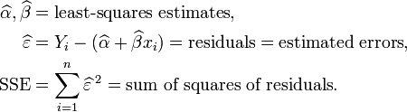
$\begin{align} \widehat\alpha, \widehat\beta & = \text{least-squares estimates}, \\ \widehat\varepsilon & = Y_i - (\widehat\alpha + \widehat\beta x_i) = \text{residuals} = \text{estimated errors}, \\ \text{SSE} & = \sum_{i=1}^n \widehat\varepsilon^{\;2} = \text{sum of squares of residuals}. \end{align}$

Then

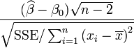
$\frac{(\widehat\beta - \beta_0)\sqrt{n-2}}{ \sqrt{\text{SSE}/\sum_{i=1}^n \left(x_i - \overline{x}\right)^2} }$

has a t-distribution with n − 2 degrees of freedom if the null hypothesis is true.

[edit] Independent two-sample t-test

[edit] Equal sample sizes, equal variance

This test is only used when both:

the two sample sizes (that is, the n or number of participants of each group) are equal;
it can be assumed that the two distributions have the same variance.

Violations of these assumptions are discussed below.

The t statistic to test whether the means are different can be calculated as follows:

$t = \frac{\bar {X}_1 - \bar{X}_2}{S_{X_1X_2} \cdot \sqrt{\frac{2}{n}}}\$

where

$\ S_{X_1X_2} = \sqrt{\frac{S_{X1}^2+S_{X2}^2}{2}} .$ ^[5]

Here $S_{X_1X_2}$ is the grand standard deviation (or pooled standard deviation), 1 = group one, 2 = group two. The denominator of t is the standard error of the difference between two means.

For significance testing, the degrees of freedom for this test is 2n − 2 where n = # of participants in each group.

[edit] Unequal sample sizes, equal variance

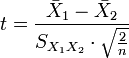
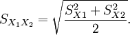
This test is used only when it can be assumed that the two distributions have the same variance. (When this assumption is violated, see below.) The t statistic to test whether the means are different can be calculated as follows:

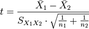
$t = \frac{\bar {X}_1 - \bar{X}_2}{S_{X_1X_2} \cdot \sqrt{\frac{1}{n_1}+\frac{1}{n_2}}}$

where

$S_{X_1X_2} = \sqrt{\frac{(n_1-1)S_{X1}^2+(n_2-1)S_{X2}^2}{n_1+n_2-2}}.$

Note that the formulae above are generalizations for the case where both samples have equal sizes (substitute n₁ and n₂ for n and you'll see).

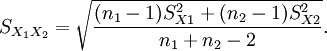
$S_{X_1X_2}$ is an estimator of the common standard deviation of the two samples: it is defined in this way so that its square is an unbiased estimator of the common variance whether or not the population means are the same. In these formulae, n = number of participants, 1 = group one, 2 = group two. n − 1 is the number of degrees of freedom for either group, and the total sample size minus two (that is, n₁ + n₂ − 2) is the total number of degrees of freedom, which is used in significance testing.

The statistical significance level associated with the t value calculated in this way is the probability that, under the null hypothesis of equal means, the absolute value of t could be that large or larger just by chance—in other words, it is a two-tailed test, testing whether the means are different when, if they are, either one may be the larger (see Press et al., 1999, p. 616).

[edit] Unequal sample sizes, unequal variance

This test is used only when the two sample sizes are unequal and the variance is assumed to be different. See also Welch's t test. The t statistic to test whether the means are different can be calculated as follows:

$t = {\overline{X}_1 - \overline{X}_2 \over s_{\overline{X}_1 - \overline{X}_2}}$

where

$s_{\overline{X}_1 - \overline{X}_2} = \sqrt{{s_1^2 \over {n}_1} + {s_2^2 \over {n}_2}}$

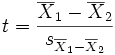
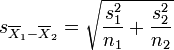
Where s² is the unbiased estimator of the variance of the two samples, n = number of participants, 1 = group one, 2 = group two. Note that in this case, $s_{\overline{X}_1 - \overline{X}_2}^2$ is not a pooled variance. For use in significance testing, the distribution of the test statistic is approximated as being an ordinary Student's t distribution with the degrees of freedom calculated using

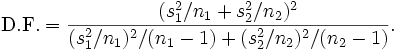
$\mathrm{D.F.} = \frac{(s_1^2/n_1 + s_2^2/n_2)^2}{(s_1^2/n_1)^2/(n_1-1) + (s_2^2/n_2)^2/(n_2-1)}.$

This is called the Welch-Satterthwaite equation. Note that the true distribution of the test statistic actually depends (slightly) on the two unknown variances: see Behrens–Fisher problem.

This test can be used as either a one-tailed or two-tailed test.

[edit] Dependent t-test for paired samples

This test is used when the samples are dependent; that is, when there is only one sample that has been tested twice (repeated measures) or when there are two samples that have been matched or "paired".

$t = \frac{\overline{X}_D - \mu_0}{{s_D}/\sqrt{N}}.$

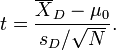
For this equation, the differences between all pairs must be calculated. The pairs are either one person's pre-test and post-test scores or between pairs of persons matched into meaningful groups (for instance drawn from the same family or age group: see table). The average (X_D) and standard deviation (s_D) of those differences are used in the equation. The constant μ₀ is non-zero if you want to test whether the average of the difference is significantly different than μ₀. The degree of freedom used is N − 1.

Number	Name	Test 1	Test 2
Example of repeated measures
1	Mike	35%	67%
2	Melanie	50%	46%
3	Melissa	90%	86%
4	Mitchell	78%	91%

Pair	Name	Age	Test
Example of matched pairs
1	Jon	35	250
1	Jane	36	340
2	Jimmy	22	460
2	Jessy	21	200

[edit] Example

A random sample of screws have weights

30.02, 29.99, 30.11, 29.97, 30.01, 29.99

Calculate a 95% confidence interval for the population's mean weight.

Assume the population is distributed as N(μ, σ²).

The samples' mean weight is 30.015 and the estimated standard deviation is 0.0497 and with five degrees of freedom.

We can look up in statistical tables that, for a confidence range of 95% and 5 degrees of freedom, the required t-value is 2.571. Note that in some tables it is necessary to look-up the 97.5% point of the student-t distribution in order to find the value appropriate to a 95% confidence interval: in other ways of presenting the table, the required value of 95% can be used to enter the table directly. Then the confidence interval is given by

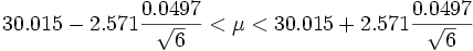
$30.015 - 2.571{0.0497 \over \sqrt{6}} < \mu < 30.015 + 2.571{0.0497 \over \sqrt{6}}$

$29.96 <\mu <30.07.\,$

If we sampled many times, our interval would capture the true mean weight 95% of the time; thus, we are 95% confident that the true mean weight of all screws will fall between 29.96 and 30.07

[edit] Alternatives to the t test

Recall that the t test can be used to test the equality of the means of two normal populations with unknown, but equal, variance.

To relax the normality assumption, a non-parametric alternative to the t test can be used, and the usual choices are:
- for independent samples, the Mann-Whitney U test
- for related samples, either the binomial test or the Wilcoxon signed-rank test
To test the equality of the means of more than two normal populations, an analysis of variance can be performed
To test the equality of the means of two normal populations with known variance, a Z-test can be performed

[edit] Multivariate testing

A generalization of Student's t statistic, called Hotelling's T-square statistic, allows for the testing of hypotheses on multiple (often correlated) measures within the same sample. For instance, a researcher might submit a number of subjects to a personality test consisting of multiple personality scales (e.g. the Big Five). Because measures of this type are usually highly correlated, it is not advisable to conduct separate univariate t-tests to test hypotheses, as these would neglect the covariance among measures and inflate the chance of falsely rejecting at least one hypothesis (Type I error). In this case a single multivariate test is preferable for hypothesis testing. Hotelling's T² statistic follows a T² distribution. However, in practice the distribution is rarely used, and instead converted to an F distribution.

[edit] One-sample T² test

For a one-sample multivariate test, the hypothesis is that the mean vector ( ${\mathbf\mu}$ ) is equal to a given vector ( ${\mathbf\mu_0}$ ). The test statistic is defined as:

$T^2=n(\overline{\mathbf x}-{\mathbf\mu_0})'{\mathbf S}^{-1}(\overline{\mathbf x}-{\mathbf\mu_0}).$

where $n$ is the sample size, $\overline{\mathbf x}$ is the vector of column means and ${\mathbf S}$ is a $m\times m$ sample covariance matrix.

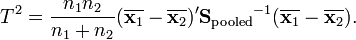
[edit] Two-sample T² test

For a two-sample multivariate test, the hypothesis is that the mean vectors ( ${\mathbf\mu_1}$ , ${\mathbf\mu_2}$ ) of two samples are equal. The test statistic is defined as

$T^2 = \frac{n_1 n_2}{n_1+n_2}(\overline{\mathbf x_1}-\overline{\mathbf x_2})'{\mathbf S_\text{pooled}}^{-1}(\overline{\mathbf x_1}-\overline{\mathbf x_2}).$

[edit] Implementations

Most spreadsheet programs and statistics packages, such as Microsoft Excel, SPSS, DAP, gretl, R and PSPP include implementations of Student's t-test.

[edit] Notes

^ Richard Mankiewicz, The Story of Mathematics (Princeton University Press), p.158.
^ ^a ^b O'Connor, John J.; Robertson, Edmund F., "Student's t-test", MacTutor History of Mathematics archive
^ Raju TN (2005). "William Sealy Gosset and William A. Silverman: two "students" of science". Pediatrics 116 (3): 732–5. doi:10.1542/peds.2005-1134. PMID 16140715.
^ ^a ^b Fadem, Barbara (2008). High-Yield Behavioral Science (High-Yield Series). Hagerstwon, MD: Lippincott Williams & Wilkins. ISBN 0-7817-8258-9.
^ BUSSAB, W.O., MORETTIN, P.A., Estatística Básica, 4ª Ed., São Paulo, 1987.

[edit] References

O'Mahony, Michael (1986). Sensory Evaluation of Food: Statistical Methods and Procedures. CRC Press. pp. 487. ISBN 0-824-77337-3.

Press, William H.; Saul A. Teukolsky, William T. Vetterling, Brian P. Flannery (1992). Numerical Recipes in C: The Art of Scientific Computing. Cambridge University Press. pp. p. 616. ISBN 0-521-43108-5. http://www.nr.com/.

[edit] External links

Statistics portal

Wikiversity has learning materials about t-test

A conceptual article on the Student's t-test

[edit] Online calculators

Online T-Test Calculator
2 Sample T-Test Calculator
GraphPad's Paired/Unpaired/Welch T-Test Calculator
OpenEpi software program

[0] Richard Mankiewicz, The Story of Mathematics (Princeton University Press), p.158.

[Gossett-1] O'Connor, John J.; Robertson, Edmund F., "Student's t-test", MacTutor History of Mathematics archive

[2] Raju TN (2005). "William Sealy Gosset and William A. Silverman: two "students" of science". Pediatrics 116 (3): 732–5. doi:10.1542/peds.2005-1134. PMID 16140715.

[fadem-3] Fadem, Barbara (2008). High-Yield Behavioral Science (High-Yield Series). Hagerstwon, MD: Lippincott Williams & Wilkins. ISBN 0-7817-8258-9.

[4] BUSSAB, W.O., MORETTIN, P.A., Estatística Básica, 4ª Ed., São Paulo, 1987.

[1]

[2]

[3]

[4]

[5]

Student's t-test

From Wikipedia, the free encyclopedia

Contents

[edit] History

[edit] Uses

[edit] Assumptions

[edit] Determining type

[edit] Calculations

[edit] Independent one-sample t-test

[edit] Slope of a regression line

[edit] Independent two-sample t-test

[edit] Equal sample sizes, equal variance

[edit] Unequal sample sizes, equal variance

[edit] Unequal sample sizes, unequal variance

[edit] Dependent t-test for paired samples

[edit] Example

[edit] Alternatives to the t test

[edit] Multivariate testing

[edit] One-sample T² test

[edit] Two-sample T² test

[edit] Implementations

[edit] Notes

[edit] References

[edit] External links

[edit] Online calculators

Views

Personal tools

Navigation

Search

Interaction

Toolbox

Languages

Student's t-test

From Wikipedia, the free encyclopedia

Contents

[edit] History

[edit] Uses

[edit] Assumptions

[edit] Determining type

[edit] Calculations

[edit] Independent one-sample t-test

[edit] Slope of a regression line

[edit] Independent two-sample t-test

[edit] Equal sample sizes, equal variance

[edit] Unequal sample sizes, equal variance

[edit] Unequal sample sizes, unequal variance

[edit] Dependent t-test for paired samples

[edit] Example

[edit] Alternatives to the t test

[edit] Multivariate testing

[edit] One-sample T 2 test

[edit] Two-sample T 2 test

[edit] Implementations

[edit] Notes

[edit] References

[edit] External links

[edit] Online calculators

Views

Personal tools

Navigation

Search

Interaction

Toolbox

Languages

[edit] One-sample T² test

[edit] Two-sample T² test