Uncertainty principle
From Wikipedia, the free encyclopedia

In quantum physics, the Heisenberg uncertainty principle states that certain physical quantities, like position and momentum, cannot both have precise values at the same time. The narrower the probability distribution for one, the wider it is for the other.
In quantum mechanics, a particle is described by a wave. The position is where the wave is concentrated and the momentum is the wavelength. The position is uncertain to the degree that the wave is spread out, and the momentum is uncertain to the degree that the wavelength is ill-defined.
The only kind of wave with a definite position is concentrated at one point, and such a wave has an indefinite wavelength. Conversely, the only kind of wave with a definite wavelength is an infinite regular periodic oscillation over all space, which has no definite position. So in quantum mechanics, there are no states that describe a particle with both a definite position and a definite momentum. The more precise the position, the less precise the momentum.
The uncertainty principle can be restated in terms of measurements, which involves collapse of the wavefunction. When the position is measured, the wavefunction collapses to a narrow bump near the measured value, and the momentum wavefunction becomes spread out. The particle's momentum is left uncertain by an amount inversely proportional to the accuracy of the position measurement. The amount of left-over uncertainty can never be reduced below the limit set by the uncertainty principle, no matter what the measurement process.
This means that the uncertainty principle is related to the observer effect, with which it is often conflated. The uncertainty principle sets a lower limit to how small the momentum disturbance in an accurate position experiment can be, and vice versa for momentum experiments.
A mathematical statement of the principle is that every quantum state has the property that the root-mean-square (RMS) deviation of the position from its mean (the standard deviation of the X-distribution):

times the RMS deviation of the momentum from its mean (the standard deviation of P):

can never be smaller than a fixed fraction of Planck's constant:

Any measurement of the position with accuracy  collapses the quantum state making the standard deviation of the momentum
  larger than
  .
.
Contents |
[edit] Historical introduction
Werner Heisenberg formulated the uncertainty principle in Niels Bohr's institute at Copenhagen, while working on the mathematical foundations of quantum mechanics.
In 1925, following pioneering work with Hendrik Kramers, Heisenberg developed matrix mechanics, which replaced the ad-hoc old quantum theory with modern quantum mechanics. The central assumption was that the classical motion was not precise at the quantum level, and electrons in an atom did not travel on sharply defined orbits. Rather, the motion was smeared out in a strange way: the time Fourier transform only involving those frequencies that could be seen in quantum jumps.
Heisenberg's paper did not admit any unobservable quantities like the exact position of the electron in an orbit at any time; he only allowed the theorist to talk about the Fourier components of the motion. Since the Fourier components were not defined at the classical frequencies, they could not be used to construct an exact trajectory, so that the formalism could not answer certain overly precise questions about where the electron was or how fast it was going.
The most striking property of Heisenberg's infinite matrices for the position and momentum is that they do not commute. His central result was the canonical commutation relation:
![[X,P] = X P - P X = i \hbar \,](http://upload.wikimedia.org/math/9/a/b/9ab5bbc4a1b8b6309c6d7f9b68520499.png)
and this result does not have a clear physical interpretation.
In March 1926, working in Bohr's institute, Heisenberg formulated the principle of uncertainty thereby laying the foundation of what became known as the Copenhagen interpretation of quantum mechanics. Heisenberg showed that the commutation relations implies an uncertainty, or in Bohr's language a complementarity. Any two variables that do not commute cannot be measured simultaneously—the more precisely one is known, the less precisely the other can be known.
One way to understand the complementarity between position and momentum is by wave-particle duality. If a particle described by a plane wave passes through a narrow slit in a wall like a water-wave passing through a narrow channel, the particle diffracts and its wave comes out in a range of angles. The narrower the slit, the wider the diffracted wave and the greater the uncertainty in momentum afterwards. The laws of diffraction require that the spread in angle Δθ is about λ / d, where d is the slit width and λ is the wavelength. From de Broglie's relation, the size of the slit and the range in momentum of the diffracted wave are related by Heisenberg's rule:

In his celebrated paper (1927), Heisenberg established this expression as the minimum amount of unavoidable momentum disturbance caused by any position measurement[1], but he did not give a precise definition for the uncertainties Δx and Δp. Instead, he gave some plausible estimates in each case separately. In his Chicago lecture[2] he refined his principle:
|
 |
| But it was Kennard[3] in 1927 who first proved the modern inequality: | |
|
 |
where  , and σx, σp are the standard deviations of position and momentum. Heisenberg himself only proved relation (2) for the special case of Gaussian states.[2].
[edit] Uncertainty principle and observer effect
The uncertainty principle is often explained as the statement that the measurement of position necessarily disturbs a particle's momentum, and vice versa—i.e., that the uncertainty principle is a manifestation of the observer effect.
This common explanation is incorrect, because the uncertainty principle is not caused by observer-effect measurement disturbance. For example, sometimes the measurement can be performed far away in ways which cannot possibly "disturb" the particle in any classical sense. But the distant measurement (of momentum for instance) still causes the waveform to collapse and make determination of (position for instance) impossible. This queer mechanism of quantum mechanics is the basis of quantum cryptography, where the measurement of a value on one of two entangled particles at one location forces, via the uncertainty principle, a property of a distant particle to become indeterminate and hence unmeasurable. If two photons are emitted in opposite directions from the decay of positronium, the momenta of the two photons are, by definition, opposite. By measuring the momentum of one particle, the momentum of the other is determined, making its position indeterminate. This case is subtler, because it is impossible to introduce more uncertainties by measuring a distant particle, but it is possible to restrict the uncertainties in different ways, with different statistical properties, depending on what property of the distant particle you choose to measure. By restricting the uncertainty in p to be very small by a distant measurement, the remaining uncertainty in x stays large. (This example was actually the basis of Albert Einstein's important suggestion of the EPR paradox in 1935.)
This disturbance explanation is also incorrect because it makes it seem that the disturbances are somehow conceptually avoidable — that there are states of the particle with definite position and momentum, but the experimental devices we have could never be good enough to produce those states. In fact, states with both definite position and momentum just do not exist in quantum mechanics, so it is not the measurement equipment that is at fault.
It is also misleading in another way, because sometimes it is a failure to measure the particle that produces the disturbance. For example, if a perfect photographic film contains a small hole, and an incident photon is not observed, then its momentum becomes uncertain by a large amount. By not observing the photon, we discover indirectly that it went through the hole, revealing the photon's position.
But Heisenberg did not focus on the mathematics of quantum mechanics, he was primarily concerned with establishing that the uncertainty is actually a property of the world — that it is in fact physically impossible to measure the position and momentum of a particle to a precision better than that allowed by quantum mechanics. To do this, he used physical arguments based on the existence of quanta, but not the full quantum mechanical formalism.
This was a surprising prediction of quantum mechanics, and not yet accepted. Many people would have considered it a flaw that there are no states of definite position and momentum. Heisenberg was trying to show this was not a bug, but a feature—a deep, surprising aspect of the universe. To do this, he could not just use the mathematical formalism, because it was the mathematical formalism itself that he was trying to justify.
[edit] Heisenberg's microscope

One way in which Heisenberg originally argued for the uncertainty principle is by using an imaginary microscope as a measuring device.[2] He imagines an experimenter trying to measure the position and momentum of an electron by shooting a photon at it.
If the photon has a short wavelength, and therefore a large momentum, the position can be measured accurately. But the photon scatters in a random direction, transferring a large and uncertain amount of momentum to the electron. If the photon has a long wavelength and low momentum, the collision doesn't disturb the electron's momentum very much, but the scattering will reveal its position only vaguely.
If a large aperture is used for the microscope, the electron's location can be well resolved (see Rayleigh criterion); but by the principle of conservation of momentum, the transverse momentum of the incoming photon and hence the new momentum of the electron resolves poorly. If a small aperture is used, the accuracy of the two resolutions is the other way around.
The trade-offs imply that no matter what photon wavelength and aperture size are used, the product of the uncertainty in measured position and measured momentum is greater than or equal to a lower bound, which is up to a small numerical factor equal to Planck's constant.[4] Heisenberg did not care to formulate the uncertainty principle as an exact bound, and preferred to use it as a heuristic quantitative statement, correct up to small numerical factors.
[edit] Critical reactions
The Copenhagen interpretation of quantum mechanics and Heisenberg's Uncertainty Principle were in fact seen as twin targets by detractors who believed in an underlying determinism and realism. Within the Copenhagen interpretation of quantum mechanics, there is no fundamental reality the quantum state describes, just a prescription for calculating experimental results. There is no way to say what the state of a system fundamentally is, only what the result of observations might be.
Albert Einstein believed that randomness is a reflection of our ignorance of some fundamental property of reality, while Niels Bohr believed that the probability distributions are fundamental and irreducible, and depend on which measurements we choose to perform. Einstein and Bohr debated the uncertainty principle for many years.
[edit] Einstein's slit
The first of Einstein's thought experiments challenging the uncertainty principle went as follows:
- Consider a particle passing through a slit of width d. The slit introduces an uncertainty in momentum of approximately h/d because the particle passes through the wall. But let us determine the momentum of the particle by measuring the recoil of the wall. In doing so, we find the momentum of the particle to arbitrary accuracy by conservation of momentum.
Bohr's response was that the wall is quantum mechanical as well, and that to measure the recoil to accuracy ΔP the momentum of the wall must be known to this accuracy before the particle passes through. This introduces an uncertainty in the position of the wall and therefore the position of the slit equal to h / ΔP, and if the wall's momentum is known precisely enough to measure the recoil, the slit's position is uncertain enough to disallow a position measurement.
A similar analysis with particles diffracting through multiple slits is given by Richard Feynman[5].
[edit] Einstein's box
Another of Einstein's thought experiments was designed to challenge the time/energy uncertainty principle. It is very similar to the slit experiment in space, except here the narrow window the particle passes through is in time:
- Consider a box filled with light. The box has a shutter that a clock opens and quickly closes at a precise time, and some of the light escapes. We can set the clock so that the time that the energy escapes is known. To measure the amount of energy that leaves, Einstein proposed weighing the box just after the emission. The missing energy lessens the weight of the box. If the box is mounted on a scale, it is naively possible to adjust the parameters so that the uncertainty principle is violated.
Bohr spent a day considering this setup, but eventually realized that if the energy of the box is precisely known, the time the shutter opens at is uncertain. If the case, scale, and box are in a gravitational field then, in some cases, it is the uncertainty of the position of the clock in the gravitational field that alter the ticking rate. This can introduce the right amount of uncertainty. This was ironic, because it was Einstein himself who first discovered gravity's effect on clocks.
[edit] EPR measurements
Bohr was compelled to modify his understanding of the uncertainty principle after another thought experiment by Einstein. In 1935, Einstein, Podolski and Rosen (see EPR paradox) published an analysis of widely separated entangled particles. Measuring one particle, Einstein realized, would alter the probability distribution of the other, yet here the other particle could not possibly be disturbed. This example led Bohr to revise his understanding of the principle, concluding that the uncertainty was not caused by a direct interaction.[6]
But Einstein came to much more far-reaching conclusions from the same thought experiment. He believed as "natural basic assumption" that a complete description of reality would have to predict the results of experiments from "locally changing deterministic quantities", and therefore would have to include more information than the maximum possible allowed by the uncertainty principle.
In 1964 John Bell showed that this assumption can be falsified, since it would imply a certain inequality between the probability of different experiments. Experimental results confirm the predictions of quantum mechanics, ruling out Einstein's basic assumption that led him to the suggestion of his hidden variables. (Ironically this is one of the best examples for Karl Popper's philosophy of invalidation of a theory by falsification-experiments, i.e. here Einstein's "basic assumption" became falsified by experiments based on Bells inequalities; for the objections of Karl Popper against the Heisenberg inequality itself, see below.)
While it is possible to assume that quantum mechanical predictions are due to nonlocal hidden variables, and in fact David Bohm invented such a formulation, this is not a satisfactory resolution for the vast majority of physicists. The question of whether a random outcome is predetermined by a nonlocal theory can be philosophical, and potentially intractable. If the hidden variables are not constrained, they could just be a list of random digits that are used to produce the measurement outcomes. To make it sensible, the assumption of nonlocal hidden variables is sometimes augmented by a second assumption — that the size of the observable universe puts a limit on the computations that these variables can do. A nonlocal theory of this sort predicts that a quantum computer encounters fundamental obstacles when it tries to factor numbers of approximately 10,000 digits or more, an achievable task in quantum mechanics[7].
[edit] Popper's criticism
Karl Popper criticized Heisenberg's form of the uncertainty principle, that a measurement of position disturbs the momentum, based on the following observation: if a particle with definite momentum passes through a narrow slit, the diffracted wave has some amplitude to go in the original direction of motion. If the momentum of the particle is measured after it goes through the slit, there is always some probability, however small, that the momentum will be the same as it was before.
Popper thinks of these rare events as falsifications of the uncertainty principle in Heisenberg's original formulation. To preserve the principle, he concludes that Heisenberg's relation does not apply to individual particles or measurements, but only to many identically prepared particles, called ensembles. Popper's criticism applies to nearly all probabilistic theories, since a probabilistic statement requires many measurements to either verify or falsify.
Popper's criticism does not trouble physicists who subscribe to Copenhagen interpretation. Popper's presumption is that the measurement is revealing some preexisting information about the particle, the momentum, which the particle already possesses. According to Copenhagen interpretation the quantum mechanical description the wavefunction is not a reflection of ignorance about the values of some more fundamental quantities, it is the complete description of the state of the particle. In this philosophical view, Popper's example is not a falsification, since after the particle diffracts through the slit and before the momentum is measured, the wavefunction is changed so that the momentum is still as uncertain as the principle demands.
[edit] Refinements
[edit] Entropic uncertainty principle
While formulating the many-worlds interpretation of quantum mechanics in 1957, Hugh Everett III discovered a much stronger formulation of the uncertainty principle[8]. In the inequality of standard deviations, some states, like the wavefunction

have a large standard deviation of position, but are actually a superposition of a small number of very narrow bumps. In this case, the momentum uncertainty is much larger than the standard deviation inequality would suggest. A better inequality uses the Shannon information content of the distribution, a measure of the number of bits learned when a random variable described by a probability distribution has a certain value.

The interpretation of I is that the number of bits of information an observer acquires when the value of x is given to accuracy ε is equal to Ix + log2(ε). The second part is just the number of bits past the decimal point, the first part is a logarithmic measure of the width of the distribution. For a uniform distribution of width Δx the information content is log2Δx. This quantity can be negative, which means that the distribution is narrower than one unit, so that learning the first few bits past the decimal point gives no information since they are not uncertain.
Taking the logarithm of Heisenberg's formulation of uncertainty in natural units.

but the lower bound is not precise.
Everett (and Hirschman[9]) conjectured that for all quantum states:

This was proven by Beckner in 1975[10].
[edit] Derivations
When linear operators A and B act on a function ψ(x), they don't always commute. A clear example is when operator B multiplies by x, while operator A takes the derivative with respect to x. Then
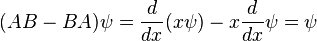
which in operator language means that

This example is important, because it is very close to the canonical commutation relation of quantum mechanics. There, the position operator multiplies the value of the wavefunction by x, while the corresponding momentum operator differentiates and multiplies by  , so that:
![[p,x] = p x - x p = -i\hbar \left( {d\over dx} x - x {d\over dx} \right) = - i \hbar](http://upload.wikimedia.org/math/5/8/6/586dfb7fa6dc5a9b076facd8d1eb3a70.png)
It is the nonzero commutator that implies the uncertainty.
For any two operators A and B:

which is a statement of the Cauchy-Schwarz inequality for the inner product of the two vectors  and
and  . The expectation value of the product AB is greater than the magnitude of its imaginary part:

and putting the two inequalities together for Hermitian operators gives a form of the Robertson-Schrödinger relation:
![\langle A^2 \rangle \langle B^2 \rangle \ge {1\over 4} |\langle [A,B]\rangle|^2](http://upload.wikimedia.org/math/e/a/9/ea96244c63616b1e0a3d9e7868a90223.png)
and the uncertainty principle is a special case.
[edit] Physical interpretation
The inequality above acquires its physical interpretation:
![\Delta_{\psi} A \, \Delta_{\psi} B \ge \frac{1}{2} \left|\left\langle\left[{A},{B}\right]\right\rangle_\psi\right|](http://upload.wikimedia.org/math/1/d/3/1d3f2c1271a50c638f3e2bccd2e72ff4.png)
where

is the mean of observable X in the state ψ and

is the standard deviation of observable X in the system state ψ.
by substituting  for A and
  for B in the general operator norm inequality, since the imaginary part of the product, the commutator, is unaffected by the shift:
![[A - \lang A\rang, B - \lang B\rang] = [ A , B ].](http://upload.wikimedia.org/math/c/1/2/c12f985e7adaf649217b038c4c613295.png)
The big side of the inequality is the product of the norms of  and
and  , which in quantum mechanics are the standard deviations of A and B. The small side is the norm of the commutator, which for the position and momentum is just
  .
.
[edit] Matrix mechanics
In matrix mechanics, the commutator of the matrices X and P is always nonzero, it is a constant multiple  of the identity matrix. This means that it is impossible for a state to have a definite values x for X and p for P, since then XP would be equal to the number xp and would equal PX.
The commutator of two matrices is unchanged when they are shifted by a constant multiple of the identity — for any two real numbers x and p
![[X-x, P- p] = [X,P] = i\hbar. \,](http://upload.wikimedia.org/math/0/f/c/0fc8bbc90a440f33a0abfc3ffcd02240.png)
Given any quantum state ψ, define the number x

to be the expected value of the position, and

to be the expected value of the momentum. The quantities  and
and  are only nonzero to the extent that the position and momentum are uncertain, to the extent that the state contains some values of X and P that deviate from the mean. The expected value of the commutator
![\langle \psi| \hat X \hat P - \hat P \hat X |\psi\rangle = \langle \psi| [ \hat X, \hat P ] |\psi\rangle = i \hbar \langle \psi|\psi \rangle = i \hbar
\,](http://upload.wikimedia.org/math/2/4/5/245ec0a37be10fcd7334f8321475c072.png)
can only be nonzero if the deviations in X in the state  times the deviations in P are large enough.
The size of the typical matrix elements can be estimated by summing the squares over the energy states  :
:

and this is equal to the square of the deviation, matrix elements have a size approximately given by the deviation.
So, to produce the canonical commutation relations, the product of the deviations in any state has to be about .

This heuristic estimate can be made into a precise inequality using the Cauchy-Schwartz inequality, exactly as before. The inner product of the two vectors in parentheses:
is bounded above by the product of the lengths of each vector:

so, rigorously, for any state:

the real part of a matrix M is  , so that the real part of the product of two Hermitian matrices
  is:
is:

while the imaginary part is
![\mathrm{Im} (\hat X \hat P) = {\hat X \hat P - \hat P \hat X \over 2i } = { [\hat X,\hat P] \over 2i }= { \hbar \over 2}.](http://upload.wikimedia.org/math/2/b/0/2b0cbb22a539c86af1dc9202f476f7d4.png)
The magnitude of  is bigger than the magnitude of its imaginary part, which is the expected value of the imaginary part of the matrix:

Note that the uncertainty product is for the same reason bounded below by the expected value of the anticommutator, which adds a term to the uncertainty relation. The extra term is not as useful for the uncertainty of position and momentum, because it has zero expected value in a gaussian wavepacket, like the ground state of a harmonic oscillator. The anticommutator term is useful for bounding the uncertainty of spin operators though.
[edit] Wave mechanics
In Schrödinger's wave mechanics, the quantum mechanical wavefunction contains information about both the position and the momentum of the particle. The position of the particle is where the wave is concentrated, while the momentum is the typical wavelength.
The wavelength of a localized wave cannot be determined very well. If the wave extends over a region of size L and the wavelength is approximately λ, the number of cycles in the region is approximately L / λ. The inverse of the wavelength can be changed by about 1 / L without changing the number of cycles in the region by a full unit, and this is approximately the uncertainty in the inverse of the wavelength,

This is an exact counterpart to a well known result in signal processing — the shorter a pulse in time, the less well defined the frequency. The width of a pulse in frequency space is inversely proportional to the width in time. It is a fundamental result in Fourier analysis, the narrower the peak of a function, the broader the Fourier transform.
Multiplying by h, and identifying ΔP = hΔ(1 / λ), and identifying ΔX = L.

The uncertainty Principle can be seen as a theorem in Fourier analysis: the standard deviation of the squared absolute value of a function, times the standard deviation of the squared absolute value of its Fourier transform, is at least 1/(16π2) (Folland and Sitaram, Theorem 1.1).
An instructive example is the (unnormalized) gaussian wave-function

The expectation value of X is zero by symmetry, and so the variance is found by averaging X2 over all positions with the weight ψ(x)2, careful to divide by the normalization factor.

The Fourier transform of the Gaussian is the wavefunction in k space, where k is the wavenumber and is related to the momentum by DeBroglie's relation  :
:

The last integral does not depend on p, because there is a continuous change of variables  which removes the dependence, and this deformation of the integration path in the complex plane does not pass through any singularities. So up to normalization, the answer is again a Gaussian.

The width of the distribution in k is found in the same way as before, and the answer just flips A to 1/A.

so that for this example

which shows that the uncertainty relation inequality is tight. There are wavefunctions that saturate the bound.
[edit] Symplectic geometry
| This section requires expansion. |
In mathematical terms, conjugate variables forms part of a symplectic basis, and the uncertainty principle corresponds to the symplectic form.
[edit] Robertson–Schrödinger relation
Given any two Hermitian operators A and B, and a system in the state ψ, there are probability distributions for the value of a measurement of A and B, with standard deviations ΔψA and ΔψB. Then
![\Delta_\psi A \, \Delta_\psi B \geq \sqrt{ \frac{1}{4}\left|\left\langle\left[{A},{B}\right]\right\rangle_\psi\right|^2
+{1\over 4} \left|\left\langle\left\{ A-\langle A\rangle_\psi,B-\langle B\rangle_\psi \right\} \right\rangle_\psi \right|^2}](http://upload.wikimedia.org/math/0/9/2/092c8adc081adcc4b236e06cf01f7904.png)
where [A,B] = AB - BA is the commutator of A and B, {A,B}= AB+BA is the anticommutator, and  is the expectation value. This inequality is called the Robertson-Schrödinger relation, and includes the Heisenberg uncertainty principle as a special case. The inequality with the commutator term only was developed in 1930 by Howard Percy Robertson, and Erwin Schrödinger added the anticommutator term a little later.
[edit] Other uncertainty principles
The Robertson Schrödinger relation gives the uncertainty relation for any two observables that do not commute:
- There is an uncertainty relation between the position and momentum of an object:

- between the energy and position of a particle in a one-dimensional potential V(x):

- between angular position and angular momentum of an object with small angular uncertainty:[11]

- between two orthogonal components of the total angular momentum operator of an object:
-
- where i, j, k are distinct and Ji denotes angular momentum along the xi axis.

- between the number of electrons in a superconductor and the phase of its Ginzburg-Landau order parameter[12][13]

[edit] Energy-time uncertainty principle
One well-known uncertainty relation is not an obvious consequence of the Robertson-Schrödinger relation: the energy-time uncertainty principle.
Since energy bears the same relation to time as momentum does to space in special relativity, it was clear to many early founders, Niels Bohr among them, that the following relation holds:

but it was not obvious what Δt is, because the time at which the particle has a given state is not an operator belonging to the particle, it is a parameter describing the evolution of the system. As Lev Landau once joked "To violate the time-energy uncertainty relation all I have to do is measure the energy very precisely and then look at my watch!"
Nevertheless, Einstein and Bohr understood the heuristic meaning of the principle. A state that only exists for a short time cannot have a definite energy. To have a definite energy, the frequency of the state must accurately be defined, and this requires the state to hang around for many cycles, the reciprocal of the required accuracy.
For example, in spectroscopy, excited states have a finite lifetime. By the time-energy uncertainty principle, they do not have a definite energy, and each time they decay the energy they release is slightly different. The average energy of the outgoing photon has a peak at the theoretical energy of the state, but the distribution has a finite width called the natural linewidth. Fast-decaying states have a broad linewidth, while slow decaying states have a narrow linewidth.
The broad linewidth of fast decaying states makes it difficult to accurately measure the energy of the state, and researchers have even used microwave cavities to slow down the decay-rate, to get sharper peaks[14]. The same linewidth effect also makes it difficult to measure the rest mass of fast decaying particles in particle physics. The faster the particle decays, the less certain is its mass.
One false formulation of the energy-time uncertainty principle says that measuring the energy of a quantum system to an accuracy ΔE requires a time interval Δt > h / ΔE. This formulation is similar to the one alluded to in Landau's joke, and was explicitly invalidated by Y. Aharonov and D. Bohm in 1961. The time Δt in the uncertainty relation is the time during which the system exists unperturbed, not the time during which the experimental equipment is turned on.
In 1936, Dirac offered a precise definition and derivation of the time-energy uncertainty relation, in a relativistic quantum theory of "events". In this formulation, particles followed a trajectory in space time, and each particle's trajectory was parametrized independently by a different proper time. The many-times formulation of quantum mechanics is mathematically equivalent to the standard formulations, but it was in a form more suited for relativistic generalization. It was the inspiration for Shin-Ichiro Tomonaga's covariant perturbation theory for quantum electrodynamics.
But a better-known, more widely-used formulation of the time-energy uncertainty principle was given only in 1945 by L. I. Mandelshtam and I. E. Tamm, as follows.[15] For a quantum system in a non-stationary state  and an observable B represented by a self-adjoint operator
  , the following formula holds:

where ΔψE is the standard deviation of the energy operator in the state , ΔψB stands for the standard deviation of the operator and  is the expectation value of in that state. Although, the second factor in the left-hand side has dimension of time, it is different from the time parameter that enters Schrödinger equation. It is a lifetime of the state with respect to the observable B. In other words, this is the time after which the expectation value changes appreciably.
[edit] See also
[edit] Notes
- ^ W. Heisenberg: Über den anschaulichen Inhalt der quantentheoretischen Kinematik und Mechanik. In: Zeitschrift für Physik. 43 1927, S. 172–198.
- ^ a b c W. Heisenberg (1930), Physikalische Prinzipien der Quantentheorie (Leipzig: Hirzel). English translation The Physical Principles of Quantum Theory (Chicago: University of Chicago Press, 1930).
- ^ E. H. Kennard, Zeitschrift für Physik 44, (1927) 326
- ^ Tipler, Paul A.; Ralph A. Llewellyn (1999). "5-5". Modern Physics (3rd ed.). W. H. Freeman and Co.. ISBN 1-5725-9164-1.
- ^ Feynman lectures on Physics, vol 3, 2-2
- ^ Walter Isaacson, "Einstein", p 452.
- ^ Gerardus 't Hooft has at times advocated this point of view.
- ^ DeWitt, Graham, The Many-Worlds Interpretation of Quantum Mechanics p. 57
- ^ I.I. Hirschman, Jr., A note on entropy. American Journal of Mathematics (1957) pp. 152–156
- ^ W. Beckner, Inequalities in Fourier analysis. Annals of Mathematics, Vol. 102, No. 6 (1975) pp. 159–182.
- ^ Franke-Arnold, Sonja (2004). "Uncertainty principle for angular position and angular momentum" ([dead link] – Scholar search). New Journal of Physics 6: 103. doi:10.1088/1367–2630/6/1/103 (inactive 2009-02-14). http://www.iop.org/EJ/article/1367–2630/6/1/103/njp4_1_103.html.
- ^ Likharev, K.K.; A.B. Zorin (1985). "Theory of Bloch-Wave Oscillations in Small Josephson Junctions". J. Low Temp. Phys. 59 (3/4): 347–382. doi:.
- ^ Anderson, P.W. (1964), "Special Effects in Superconductivity", in Caianiello, E.R., Lectures on the Many-Body Problem, Vol. 2, New York: Academic Press
- ^ Gabrielse, Gerald; H. Dehmelt (1985). "Observation of Inhibited Spontaneous Emission". Physical Review Letters 55: 67–70. doi:.
- ^ L. I. Mandelshtam, I. E. Tamm, The uncertainty relation between energy and time in nonrelativistic quantum mechanics, 1945
[edit] References
- W. Heisenberg, "Über den anschaulichen Inhalt der quantentheoretischen Kinematik und Mechanik", Zeitschrift für Physik, 43 1927, pp. 172–198. English translation: J. A. Wheeler and H. Zurek, Quantum Theory and Measurement Princeton Univ. Press, 1983, pp. 62–84.
- L. I. Mandelshtam, I. E. Tamm "The uncertainty relation between energy and time in nonrelativistic quantum mechanics", Izv. Akad. Nauk SSSR (ser. fiz.) 9, 122-128 (1945). English translation: J. Phys. (USSR) 9, 249-254 (1945).
- Folland, Gerald; Sitaram, Alladi (May 1997). "The Uncertainty Principle: A Mathematical Survey" (PDF). Journal of Fourier Analysis and Applications 3 (3): 207–238. doi:. MR98f:42006. http://www.springerlink.com/content/f7492v6374716m4g/fulltext.pdf.
- Q. Zheng and T. Kobayashi, Quantum Optics as a Relativistic Theory of Light; Physics Essays 9 (1996) 447. Annual Report, Department of Physics, School of Science, University of Tokyo (1992) 240.
[edit] External links
- Annotated pre-publication proof sheet of Uber den anschaulichen Inhalt der quantentheoretischen Kinematik und Mechanik, March 23, 1927.
- Matter as a Wave - a chapter from an online textbook
- The Uncertainty Relations: Description, Applications on Project PHYSNET
- Quantum mechanics: Myths and facts
- Stanford Encyclopedia of Philosophy entry
- aip.org: Quantum mechanics 1925–1927 - The uncertainty principle
- Eric Weisstein's World of Physics - Uncertainty principle
- Fourier Transforms and Uncertainty at MathPages
- Schrödinger equation from an exact uncertainty principle
- John Baez on the time-energy uncertainty relation
- The time-energy certainty relation - It is shown that something opposite to the time-energy uncertainty relation is true.
- The certainty principle

