Transformation matrix

From Wikipedia, the free encyclopedia

In linear algebra, linear transformations can be represented by matrices. If T is a linear transformation mapping Rⁿ to R^m and x is a column vector with n entries, then

$T( \vec x ) = \mathbf{A} \vec x$

for some m×n matrix A, called the transformation matrix of T.

[edit] Uses

Matrices allow arbitrary linear transformations to be represented in a consistent format, suitable for computation. This also allows transformations to be concatenated easily (by multiplying their matrices).

Linear transformations are not the only ones that can be represented by matrices. Using homogeneous coordinates, both affine transformations and perspective projections on Rⁿ can be represented as linear transformations on RPⁿ⁺¹ (that is, n+1-dimensional real projective space). For this reason, 4x4 transformation matrices are widely used in 3D computer graphics.

3-by-3 or 4-by-4 transformation matrices containing homogeneous coordinates are often called, somewhat improperly, "homogeneous transformation matrices". However, the transformations they represent are, in most cases, definitely non-homogeneous and non-linear (like translation, roto-translation or perspective projection). And even the matrices themselves look rather heterogeneous, i.e. composed of different kinds of elements (see below). Since they are multi-purpose transformation matrices, capable of representing both affine and projective transformations, they might be called "general transformation matrices", or, depending on the application, "affine transformation" or "perspective projection" matrices. Moreover, since the homogeneous coordinates describe a projective vector space, they can also be called "projective space transformation matrices".

[edit] Finding the matrix of a transformation

If one has a linear transformation $T (x)$ in functional form, it is easy to determine the transformation matrix A by simply transforming each of the vectors of the standard basis by T and then inserting the results into the columns of a matrix. In other words,

$\mathbf{A} = \begin{bmatrix} T( \vec e_1 ) & T( \vec e_2 ) & \cdots & T( \vec e_n ) \end{bmatrix}$

For example, the function $T (x) = 5 x$ is a linear transformation. Applying the above process (suppose that n = 2 in this case) reveals that

$T( \vec x ) = 5 \vec x = \begin{bmatrix} 5 && 0 \\ 0 && 5 \end{bmatrix} \vec x$

[edit] Examples in 2D graphics

Most common geometric transformations that keep the origin fixed are linear, including rotation, scaling, shearing, reflection, and orthogonal projection; if an affine transformation is not a pure translation it keeps some point fixed, and that point can be chosen as origin to make the transformation linear. In two dimensions, linear transformations can be represented using a 2×2 transformation matrix.

[edit] Rotation

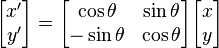
For rotation by an angle θ counterclockwise about the origin, the functional form is $x' = x cosθ - y sinθ$ and $y' = x sinθ + y cosθ$ . Written in matrix form, this becomes:

$\begin{bmatrix} x' \\ y' \end{bmatrix} = \begin{bmatrix} \cos \theta & -\sin\theta \\ \sin \theta & \cos \theta \end{bmatrix} \begin{bmatrix} x \\ y \end{bmatrix}$

Similarly, for a rotation clockwise about the origin, the functional form is $x' = x cosθ + y sinθ$ and $y' = - x sinθ + y cosθ$ and the matrix form is:

$\begin{bmatrix} x' \\ y' \end{bmatrix} = \begin{bmatrix} \cos \theta & \sin\theta \\ -\sin \theta & \cos \theta \end{bmatrix} \begin{bmatrix} x \\ y \end{bmatrix}$

[edit] Scaling

For scaling (that is, enlarging or shrinking), we have $x' = s_x \cdot x$ and $y' = s_y \cdot y$ . The matrix form is:

$\begin{bmatrix} x' \\ y' \end{bmatrix} = \begin{bmatrix} s_x & 0 \\ 0 & s_y \end{bmatrix} \begin{bmatrix} x \\ y \end{bmatrix}$

[edit] Shearing

For shear mapping (visually similar to slanting), there are two possibilities. For a shear parallel to the x axis has $x' = x + k y$ and $y' = y$ ; the shear matrix, applied to column vectors, is:

$\begin{bmatrix} x' \\ y' \end{bmatrix} = \begin{bmatrix} 1 & k \\ 0 & 1 \end{bmatrix} \begin{bmatrix} x \\ y \end{bmatrix}$

A shear parallel to the y axis has $x' = x$ and $y' = y + k x$ , which has matrix form:

$\begin{bmatrix} x' \\ y' \end{bmatrix} = \begin{bmatrix} 1 & 0 \\ k & 1 \end{bmatrix} \begin{bmatrix} x \\ y \end{bmatrix}$

[edit] Reflection

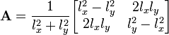
To reflect a vector about a line that goes through the origin, let (l_x, l_y) be a vector in the direction of the line:

$\mathbf{A} = \frac{1}{l_x^2 + l_y^2} \begin{bmatrix} l_x^2 - l_y^2 & 2 l_x l_y \\ 2 l_x l_y & l_y^2 - l_x^2 \end{bmatrix}$

A reflection about a line that does not go through the origin is not a linear transformation; it is an affine transformation.

To reflect a point through a plane $a x + b y + c z = 0$ you can use the equation $I - 2 N N T$ . Where I is the identity matrix and N is the unit vector for the surface normal of the plane. The transformation matrix received will be:

$\begin{bmatrix} 1 - 2 a^2 & - 2 a b & - 2 a c \\ - 2 a b & 1 - 2 b^2 & - 2 b c \\ - 2 a c & - 2 b c & 1 - 2c^2 \end{bmatrix}$

Note that this technique only works if the plane runs through the origin: if it does not, an affine transformation is required.

[edit] Orthogonal projection

To project a vector orthogonally onto a line that goes through the origin, let (u_x, u_y) be a vector in the direction of the line. Then use the transformation matrix:

$\mathbf{A} = \frac{1}{u_x^2 + u_y^2} \begin{bmatrix} u_x^2 & -u_x u_y \\ -u_x u_y & u_y^2 \end{bmatrix}$

As with reflections, the orthogonal projection onto a line that does not pass through the origin is an affine, not linear, transformation.

Parallel projections are also linear transformations and can be represented simply by a matrix. However, perspective projections are not, and to represent these with a matrix, homogeneous coordinates must be used.

[edit] Composing and inverting transformations

One of the main motivations for using matrices to represent linear transformations is that transformations can then be easily composed (combined) and inverted.

Composition is accomplished by matrix multiplication. If A and B are the matrices of two linear transformations, then the effect of applying first A and then B to a vector x is given by:

$\mathbf{B}(\mathbf{A} \vec x ) = (\mathbf{BA}) \vec x$

In other words, the matrix of the combined transformation A followed by B is simply the product of the individual matrices. Note that the multiplication is done in the opposite order from the English sentence: the matrix of "A followed by B" is BA, not AB.

A consequence of the ability to compose transformations by multiplying their matrices is that transformations can also be inverted by simply inverting their matrices. So, A^-1 represents the transformation that "undoes" A.

[edit] Other kinds of transformations

[edit] Affine transformations

To represent affine transformations with matrices, we must use homogeneous coordinates. This means representing a 2-vector (x, y) as a 3-vector (x, y, 1), and similarly for higher dimensions. Using this system, translation can be expressed with matrix multiplication. The functional form $x' = x + t x$ ; $y' = y + t y$ becomes:

$\begin{bmatrix} x' \\ y' \\ 1 \end{bmatrix} = \begin{bmatrix} 1 & 0 & t_x \\ 0 & 1 & t_y \\ 0 & 0 & 1 \end{bmatrix} \begin{bmatrix} x \\ y \\ 1 \end{bmatrix}.$

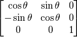
All ordinary linear transformations are included in the set of affine transformations, and can be described as a simplified form of affine transformations. Hence, any linear transformation can be also represented by a general transformation matrix. The latter is obtained by expanding the corresponding linear transformation matrix by one row and column, filling the extra space with zeros except for the lower-right corner, which must be set to 1. For example, the rotation matrix from above becomes:

$\begin{bmatrix} \cos \theta & \sin \theta & 0 \\ -\sin \theta & \cos \theta & 0 \\ 0 & 0 & 1 \end{bmatrix}$

Using transformation matrices containing homogeneous coordinates, translations can be seamlessly intermixed with all other types of transformations. The reason is that the real plane is mapped to the w = 1 plane in real projective space, and so translation in real euclidean space can be represented as a shear in real projective space. Although a translation is a non-linear transformation in a 2-D or 3-D euclidean space described by Cartesian coordinates, it becomes, in a 3-D or 4-D projective space described by homogeneous coordinates, a simple linear transformation (a shear).

When using affine transformations, the homogeneous component of a coordinate vector (normally called w) will never be altered. One can therefore safely assume that it is always 1 and ignore it. However, this is not true when using perspective projections.

[edit] Perspective projection

See also 3D projection

Another type of transformation, of importance in 3D computer graphics, is the perspective projection. Whereas parallel projections are used to project points onto the image plane along parallel lines, the perspective projection projects points onto the image plane along lines that emanate from a single point, called the center of projection. This means that an object has a smaller projection when it is far away from the center of projection and a larger projection when it is closer.

The simplest perspective projection uses the origin as the center of projection, and z = 1 as the image plane. The functional form of this transformation is then $x' = x / z$ ; $y' = y / z$ . We can express this in homogeneous coordinates as:

$\begin{bmatrix} x_c \\ y_c \\ z_c \\ w_c \end{bmatrix} = \begin{bmatrix} 1 & 0 & 0 & 0 \\ 0 & 1 & 0 & 0 \\ 0 & 0 & 1 & 0 \\ 0 & 0 & 1 & 0 \end{bmatrix} \begin{bmatrix} x \\ y \\ z \\ 1 \end{bmatrix}$

(The result of carrying out this multiplication is that $(x c, y c, z c, w c)$ = $(x, y, z, z)$ .)

After carrying out the matrix multiplication, the homogeneous component w_c will, in general, not be equal to 1. Therefore, to map back into the real plane we must perform the homogeneous divide or perspective divide by dividing each component by w_c:

$\begin{bmatrix} x' \\ y' \\ z' \end{bmatrix} = \begin{bmatrix} x_c / w_c \\ y_c / w_c \\ z_c / w_c \end{bmatrix}$

More complicated perspective projections can be composed by combining this one with rotations, scales, translations, and shears to move the image plane and center of projection wherever they are desired.

[edit] See also

[edit] External links

The Matrix Page - practical examples in POV-Ray
Reference page - Rotation of axes
Matrices and the Transform Matrix, Understanding Flash Transform Matrices

Transformation matrix

From Wikipedia, the free encyclopedia

Contents

[edit] Uses

[edit] Finding the matrix of a transformation

[edit] Examples in 2D graphics

[edit] Rotation

[edit] Scaling

[edit] Shearing

[edit] Reflection

[edit] Orthogonal projection

[edit] Composing and inverting transformations

[edit] Other kinds of transformations

[edit] Affine transformations

[edit] Perspective projection

[edit] See also

[edit] External links

Views

Personal tools

Navigation

Search

Interaction

Toolbox

Languages