Laplace transform
From Wikipedia, the free encyclopedia
In mathematics, the Laplace transform is one of the best known and most widely used integral transforms. It is commonly used to produce an easily solvable algebraic equation from an ordinary differential equation. It has many important applications in mathematics, physics, optics, electrical engineering, control engineering, signal processing, and probability theory.
In mathematics, it is used for solving differential and integral equations. In physics, it is used for analysis of linear time-invariant systems such as electrical circuits, harmonic oscillators, optical devices, and mechanical systems. In this analysis, the Laplace transform is often interpreted as a transformation from the time-domain, in which inputs and outputs are functions of time, to the frequency-domain, where the same inputs and outputs are functions of complex angular frequency, or radians per unit time. Given a simple mathematical or functional description of an input or output to a system, the Laplace transform provides an alternative functional description that often simplifies the process of analyzing the behavior of the system, or in synthesizing a new system based on a set of specifications.
Denoted  , it is a linear operator on a function f(t) (original) with a real argument t (t ≥ 0) that transforms it to a function F(s) (image) with a complex argument s. This transformation is essentially bijective for the majority of practical uses; the respective pairs of f(t) and F(s) are matched in tables. The Laplace transform has the useful property that many relationships and operations over the originals f(t) correspond to simpler relationships and operations over the images F(s).[1]
[edit] History
The Laplace transform is named in honor of mathematician and astronomer Pierre-Simon Laplace, who used the transform in his work on probability theory.
From 1744, Leonhard Euler investigated integrals of the form:

— as solutions of differential equations but did not pursue the matter very far.[2] Joseph Louis Lagrange was an admirer of Euler and, in his work on integrating probability density functions, investigated expressions of the form:
— which some modern historians have interpreted within modern Laplace transform theory.[3][4]
These types of integrals seem first to have attracted Laplace's attention in 1782 where he was following in the spirit of Euler in using the integrals themselves as solutions of equations.[5] However, in 1785, Laplace took the critical step forward when, rather than just look for a solution in the form of an integral, he started to apply the transforms in the sense that was later to become popular. He used an integral of the form:
— akin to a Mellin transform, to transform the whole of a difference equation, in order to look for solutions of the transformed equation. He then went on to apply the Laplace transform in the same way and started to derive some of its properties, beginning to appreciate its potential power.[6]
Laplace also recognised that Joseph Fourier's method of Fourier series for solving the diffusion equation could only apply to a limited region of space as the solutions were periodic. In 1809, Laplace applied his transform to find solutions that diffused indefinitely in space.[7]
[edit] Formal definition
The Laplace transform of a function f(t), defined for all real numbers t ≥ 0, is the function F(s), defined by:

The lower limit of 0− is short notation to mean

and assures the inclusion of the entire Dirac delta function δ(t) at 0 if there is such an impulse in f(t) at 0.
The parameter s is in general complex:

This integral transform has a number of properties that make it useful for analyzing linear dynamic systems. The most significant advantage is that differentiation and integration become multiplication and division, respectively, by s. (This is similar to the way that logarithms change an operation of multiplication of numbers to addition of their logarithms.) This changes integral equations and differential equations to polynomial equations, which are much easier to solve. Once solved, use of the inverse Laplace transform reverts back to the time domain.
[edit] Bilateral Laplace transform
When one says "the Laplace transform" without qualification, the unilateral or one-sided transform is normally intended. The Laplace transform can be alternatively defined as the bilateral Laplace transform or two-sided Laplace transform by extending the limits of integration to be the entire real axis. If that is done the common unilateral transform simply becomes a special case of the bilateral transform where the definition of the function being transformed is multiplied by the Heaviside step function.
The bilateral Laplace transform is defined as follows:

[edit] Inverse Laplace transform
The inverse Laplace transform is given by the following complex integral, which is known by various names (the Bromwich integral, the Fourier-Mellin integral, and Mellin's inverse formula):

where γ is a real number so that the contour path of integration is in the region of convergence of F(s) normally requiring γ > Re(sp) for every singularity sp of F(s) and i2 = −1. If all singularities are in the left half-plane, that is Re(sp) < 0 for every sp, then γ can be set to zero and the above inverse integral formula becomes identical to the inverse Fourier transform.
An alternative formula for the inverse Laplace transform is given by Post's inversion formula.
[edit] Region of convergence
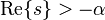
The Laplace transform F(s) typically exists for all complex numbers such that Re{s} > a, where a is a real constant which depends on the growth behavior of f(t), whereas the two-sided transform is defined in a range a < Re{s} < b. The subset of values of s for which the Laplace transform exists is called the region of convergence (ROC) or the domain of convergence. In the two-sided case, it is sometimes called the strip of convergence.
The integral defining the Laplace transform of a function may fail to exist for various reasons. For example, when the function has infinite discontinuities in the interval of integration, or when it increases so rapidly that e − pt cannot damp it sufficiently for convergence on the interval to take place. There are no specific conditions that one can check a function against to know in all cases if its Laplace transform can be taken,[citation needed] other than to say the defining integral converges. It is however possible to give theorems on cases where it may or may not be taken.
[edit] Properties and theorems
Given the functions f(t) and g(t), and their respective Laplace transforms F(s) and G(s):


the following table is a list of properties of unilateral Laplace transform:
| Time domain | Frequency domain | Comment | |
|---|---|---|---|
| Linearity |  |
 |
Can be proved using basic rules of integration. |
| Frequency differentiation |  |
 |
F' is the first derivative of F. |
| Frequency differentiation |  |
 |
More general form, (n)th derivative of F(s). |
| Differentiation |  |
 |
Obtained by integration by parts |
| Second Differentiation |  |
 |
Apply the Differentiation property to f'(t). |
| General Differentiation |  |
 |
Follow the process briefed for the Second Differentiation. |
| Frequency integration |  |
 |
|
| Integration |  |
 |
u(t) is the Heaviside step function. Note (u * f)(t) is the convolution of u(t) and f(t); it does not denote multiplication. |
| Scaling |  |
 |
|
| Frequency shifting |  |
 |
|
| Time shifting |  |
 |
u(t) is the Heaviside step function |
| Convolution |  |
 |
|
| Periodic Function |  |
 |
f(t) is a periodic function of period T so that  . This is the result of the time shifting property and the geometric series. . This is the result of the time shifting property and the geometric series. |
- Initial value theorem:
- Final value theorem:
 , if all poles of sF(s) are in the left-hand plane.
- The final value theorem is useful because it gives the long-term behaviour without having to perform partial fraction decompositions or other difficult algebra. If a function's poles are in the right hand plane (e.g. et or sin(t)) the behaviour of this formula is undefined.
[edit] Proof of the Laplace transform of a function's derivative
It is often convenient to use the differentiation property of the Laplace transform to find the transform of a function's derivative. This can be derived from the basic expression for a Laplace transform as follows:

![~~ = \left[ \frac{f(t)e^{-st}}{-s} \right]_{0^-}^{+\infty} -
\int_{0^-}^{+\infty} \frac{e^{-st}}{-s} f'(t)dt](http://upload.wikimedia.org/math/6/9/b/69b8b8059c811ca72f6290f476b91002.png) (by parts)
(by parts)
![~~ = \left[-\frac{f(0)}{-s}\right] +
\frac{1}{s}\mathcal{L}\left\{f'(t)\right\},](http://upload.wikimedia.org/math/4/4/7/4470d0e56f3d68fb882841daa6ce16ae.png)
yielding

and in the bilateral case, we have

[edit] Relationship to other transforms
[edit] Fourier transform
The continuous Fourier transform is equivalent to evaluating the bilateral Laplace transform with complex argument s = iω or s = 2πfi:
![\begin{array}{rcl}
F(\omega) & = & \mathcal{F}\left\{f(t)\right\} \\[1em]
& = & \mathcal{L}\left\{f(t)\right\}|_{s = i \omega} = F(s)|_{s = i \omega}\\[1em]
& = & \int_{-\infty}^{+\infty} e^{-\imath \omega t} f(t)\,\mathrm{d}t.\\
\end{array}](http://upload.wikimedia.org/math/f/c/3/fc32e7df55353ac581683fea747aa1b6.png)
Note that this expression excludes the scaling factor  , which is often included in definitions of the Fourier transform.
This relationship between the Laplace and Fourier transforms is often used to determine the frequency spectrum of a signal or dynamic system.
[edit] Mellin transform
The Mellin transform and its inverse are related to the two-sided Laplace transform by a simple change of variables. If in the Mellin transform

we set θ = e-t we get a two-sided Laplace transform.
[edit] Z-transform
The unilateral or one-sided Z-transform is simply the Laplace transform of an ideally sampled signal with the substitution of

- where
 is the sampling period (in units of time e.g., seconds) and
  is the sampling rate (in samples per second or hertz)
Let

be a sampling impulse train (also called a Dirac comb) and

![= \sum_{n=0}^{\infty} x(n T) \delta(t - n T) = \sum_{n=0}^{\infty} x[n] \delta(t - n T)](http://upload.wikimedia.org/math/9/5/f/95f4c1099289971353e4d712c1f57637.png)
be the continuous-time representation of the sampled  .
.
![x[n] \ \stackrel{\mathrm{def}}{=}\ x(nT) \](http://upload.wikimedia.org/math/e/6/b/e6b102901a66a7f80116631afc0ccbfa.png) are the discrete samples of .
are the discrete samples of .
The Laplace transform of the sampled signal  is
is

![\ = \int_{0^-}^{\infty} \sum_{n=0}^{\infty} x[n] \delta(t - n T) e^{-s t} \, dt](http://upload.wikimedia.org/math/f/5/8/f58438a82e01923f03754e7a73346cfe.png)
![\ = \sum_{n=0}^{\infty} x[n] \int_{0^-}^{\infty} \delta(t - n T) e^{-s t} \, dt](http://upload.wikimedia.org/math/5/9/9/599525c548908a1602887a1bd4b9ff75.png)
![\ = \sum_{n=0}^{\infty} x[n] e^{-n s T}.](http://upload.wikimedia.org/math/3/9/7/397c2b7bd71494e37cb5cde30e0591f9.png)
This is precisely the definition of the unilateral Z-transform of the discrete function ![x[n] \](http://upload.wikimedia.org/math/c/1/4/c1466b9927640af95f78274058d272d9.png)
![X(z) = \sum_{n=0}^{\infty} x[n] z^{-n}](http://upload.wikimedia.org/math/9/3/7/93762261ebf70b67ba079c79607646fa.png)
with the substitution of  .
.
Comparing the last two equations, we find the relationship between the unilateral Z-transform and the Laplace transform of the sampled signal:

The similarity between the Z and Laplace transforms is expanded upon in the theory of time scale calculus.
[edit] Borel transform
The integral form of the Borel transform is identical to the Laplace transform; indeed, these are sometimes mistakenly assumed to be synonyms. The generalized Borel transform generalizes the Laplace transform for functions not of exponential type.
[edit] Fundamental relationships
Since an ordinary Laplace transform can be written as a special case of a two-sided transform, and since the two-sided transform can be written as the sum of two one-sided transforms, the theory of the Laplace-, Fourier-, Mellin-, and Z-transforms are at bottom the same subject. However, a different point of view and different characteristic problems are associated with each of these four major integral transforms.
[edit] Table of selected Laplace transforms
The following table provides Laplace transforms for many common functions of a single variable. For definitions and explanations, see the Explanatory Notes at the end of the table.
Because the Laplace transform is a linear operator:
- The Laplace transform of a sum is the sum of Laplace transforms of each term.

- The Laplace transform of a multiple of a function, is that multiple times the Laplace transformation of that function.

The unilateral Laplace transform is only valid when t is non-negative, which is why all of the time domain functions in the table below are multiples of the Heaviside step function, u(t).
| ID | Function | Time domain |
Laplace s-domain |
Region of convergence for causal systems |
||
|---|---|---|---|---|---|---|
| 1 | ideal delay |  |
 |
|||
| 1a | unit impulse |  |
1 |  |
||
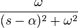
| 2 | delayed nth power with frequency shift |
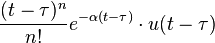 |
 |
 |
||
| 2a | nth power ( for integer n ) |
 |
 |
|
||
| 2a.1 | qth power ( for real q ) |
 |
 |
|
||
| 2a.2 | unit step |  |
 |
|
||
| 2b | delayed unit step |  |
 |
|
||
| 2c | ramp |  |
 |
|
||
| 2d | nth power with frequency shift | 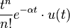 |
 |
 |
||
| 2d.1 | exponential decay |  |
 |
 |
||
| 3 | exponential approach |  |
 |
 |
||
| 4 | sine |  |
 |
|
||
| 5 | cosine |  |
 |
|
||
| 6 | hyperbolic sine |  |
 |
 |
||
| 7 | hyperbolic cosine |  |
 |
|
||
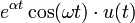
| 8 | Exponentially-decaying sine wave |
 |
 |
 |
||
| 9 | Exponentially-decaying cosine wave |
 |
 |
|
||
| 10 | nth root | ![\sqrt[n]{t} \cdot u(t)](http://upload.wikimedia.org/math/4/8/6/486b3056c275d0abfe2730f87a747f9f.png) |
 |
|
||
| 11 | natural logarithm |  |
![- { t_0 \over s} \ [ \ \ln(t_0 s)+\gamma \ ]](http://upload.wikimedia.org/math/4/5/e/45e874340427d4d5e74e12ede79de487.png) |
|
||
| 12 | Bessel function of the first kind, of order n |
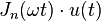 |
 |
 |
||
| 13 | Modified Bessel function of the first kind, of order n |
 |
 |
 |
||
| 14 | Bessel function of the second kind, of order 0 |
 |
 |
|
||
| 15 | Modified Bessel function of the second kind, of order 0 |
 |
||||
| 16 | Error function |  |
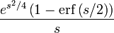 |
|
||
Explanatory notes:
|
||||||
 represents the
  represents the
  represents the
  is the
  , a real number, typically represents time,
 is the
  ,
,  ,
,  , and
, and  are
are  , is an
 [edit] s-Domain equivalent circuits and impedances
The Laplace transform is often used in circuit analysis, and simple conversions to the s-Domain of circuit elements can be made. Circuit elements can be transformed into impedances, very similar to phasor impedances.
Here is a summary of equivalents:

Note that the resistor is exactly the same in the time domain and the s-Domain. The sources are put in if there are initial conditions on the circuit elements. For example, if a capacitor has an initial voltage across it, or if the inductor has an initial current through it, the sources inserted in the s-Domain account for that.
The equivalents for current and voltage sources are simply derived from the transformations in the table above.
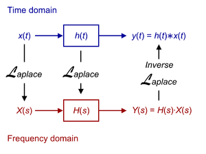
[edit] Examples: How to apply the properties and theorems
The Laplace transform is used frequently in engineering and physics; the output of a linear time invariant system can be calculated by convolving its unit impulse response with the input signal. Performing this calculation in Laplace space turns the convolution into a multiplication; the latter being easier to solve because of its algebraic form. For more information, see control theory.
The Laplace transform can also be used to solve differential equations and is used extensively in electrical engineering. The method of using the Laplace Transform to solve differential equations was developed by the English electrical engineer Oliver Heaviside.
- The following examples, derived from applications in physics and engineering, will use SI units of measure. SI is based on meters for distance, kilograms for mass, seconds for time, and amperes for electric current.
[edit] Example #1: Solving a differential equation
- The following example is based on concepts from nuclear physics.
Consider the following first-order, linear differential equation:
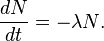
This equation is the fundamental relationship describing radioactive decay, where

represents the number of undecayed atoms remaining in a sample of a radioactive isotope at time t (in seconds), and  is the decay constant.
We can use the Laplace transform to solve this equation.
Rearranging the equation to one side, we have

Next, we take the Laplace transform of both sides of the equation:

where

and
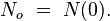
Solving, we find
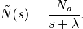
Finally, we take the inverse Laplace transform to find the general solution


which is indeed the correct form for radioactive decay.
[edit] Example #2: Deriving the complex impedance for a capacitor
- This example is based on the principles of electrical circuit theory.
The constitutive relation governing the dynamic behavior of a capacitor is the following differential equation:

where C is the capacitance (in farads) of the capacitor, i = i(t) is the electric current (in amperes) through the capacitor as a function of time, and v = v(t) is the voltage (in volts) across the terminals of the capacitor, also as a function of time.
Taking the Laplace transform of this equation, we obtain

where

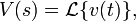 and
and

Solving for V(s) we have
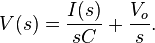
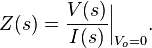
The definition of the complex impedance Z (in ohms) is the ratio of the complex voltage V divided by the complex current I while holding the initial state Vo at zero:
Using this definition and the previous equation, we find:

which is the correct expression for the complex impedance of a capacitor.
[edit] Example #3: Finding the transfer function from the impulse response
- This example is based on concepts from signal processing, and describes the dynamic behavior of a damped harmonic oscillator. See also RLC circuit.
Consider a linear time-invariant system with impulse response
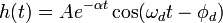
such that

where t is the time (in seconds), and

is the phase delay (in radians).
Suppose that we want to find the transfer function of the system. We begin by noting that
![h(t) = A e^{- \alpha t} \cos \left[ \omega_d (t - t_d) \right] \cdot u(t - t_d) \,](http://upload.wikimedia.org/math/6/2/0/620902c9e666086a14ee47976a65c9f3.png)
where

is the time delay of the system (in seconds), and  is the Heaviside step function.
The transfer function is simply the Laplace transform of the impulse response:


where

is the (undamped) natural frequency or resonance of the system (in radians per second).
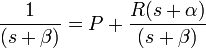
[edit] Example #4: Method of partial fraction expansion
Consider a linear time-invariant system with transfer function

The impulse response is simply the inverse Laplace transform of this transfer function:

To evaluate this inverse transform, we begin by expanding H(s) using the method of partial fraction expansion:

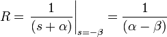
The unknown constants P and R are the residues located at the corresponding poles of the transfer function. Each residue represents the relative contribution of that singularity to the transfer function's overall shape. By the residue theorem, the inverse Laplace transform depends only upon the poles and their residues. To find the residue P, we multiply both sides of the equation by (s + α) to get
Then by letting s = − α, the contribution from R vanishes and all that is left is

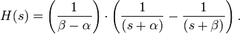
Similarly, the residue R is given by
Note that

and so the substitution of R and P into the expanded expression for H(s) gives
Finally, using the linearity property and the known transform for exponential decay (see Item #3 in the Table of Laplace Transforms, above), we can take the inverse Laplace transform of H(s) to obtain:
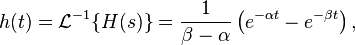
which is the impulse response of the system.
[edit] Example #5: Mixing sines, cosines, and exponentials
| Time function | Laplace transform |
|---|---|
![e^{-\alpha t}\left[ \cos{(\omega t)}+\left(\frac{\beta-\alpha}{\omega}\right)\sin{(\omega t)}\right]u(t)](http://upload.wikimedia.org/math/d/2/3/d239ce9976b7b9b57cc605fa9faf8110.png) |
 |
Starting with the Laplace transform

we find the inverse transform by first adding and subtracting the same constant α to the numerator:
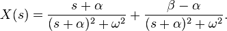
By the shift-in-frequency property, we have


![= e^{-\alpha t} \left[ \mathcal{L}^{-1} \left\{ {s \over s^2 + \omega^2} \right\} + \left( { \beta - \alpha \over \omega } \right) \mathcal{L}^{-1} \left\{ { \omega \over s^2 + \omega^2 } \right\} \right].](http://upload.wikimedia.org/math/7/f/1/7f1f9cf004477f58cc5383945d3fb666.png)
Finally, using the Laplace transforms for sine and cosine (see the table, above), we have
![x(t) = e^{-\alpha t} \left[ \cos{(\omega t)}u(t)+\left(\frac{\beta-\alpha}{\omega}\right)\sin{(\omega t)}u(t)\right].](http://upload.wikimedia.org/math/0/e/1/0e1b001ae02ae6046e274b5942249705.png)
![x(t) = e^{-\alpha t} \left[ \cos{(\omega t)}+\left(\frac{\beta-\alpha}{\omega}\right)\sin{(\omega t)}\right]u(t).](http://upload.wikimedia.org/math/4/b/5/4b576f7d61bdbc6852b2699a9ce54f7b.png)
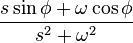
[edit] Example #6: Phase delay
| Time function | Laplace transform |
|---|---|
 |
 |
 |
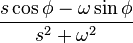 |
Starting with the Laplace transform,

we find the inverse by first rearranging terms in the fraction:


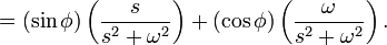
We are now able to take the inverse Laplace transform of our terms:


To simplify this answer, we must recall the trigonometric identity that

and apply it to our value for x(t):

We can apply similar logic to find that

[edit] See also
- Pierre-Simon Laplace
- Fourier transform
- Analog signal processing
- Laplace transform applied to differential equations
- Moment-generating function
[edit] References
[edit] Bibliography
[edit] Modern
- G.A. Korn and T.M. Korn, Mathematical Handbook for Scientists and Engineers, McGraw-Hill Companies; 2nd edition (June 1967). ISBN 0-0703-5370-0
- A. D. Polyanin and A. V. Manzhirov, Handbook of Integral Equations, CRC Press, Boca Raton, 1998. ISBN 0-8493-2876-4
- William McC. Siebert, Circuits, Signals, and Systems, MIT Press, Cambridge, Massachusetts, 1986. ISBN 0-262-19229-2
- Davies, Brian, Integral transforms and their applications, Third edition, Springer, New York, 2002. ISBN 0-387-95314-0
- Wolfgang Arendt, Charles J.K. Batty, Matthias Hieber, and Frank Neubrander. Vector-Valued Laplace Transforms and Cauchy Problems, Birkhäuser Basel, 2002. ISBN-10:3764365498
[edit] Historical
- Deakin, M. A. B. (1981). "The development of the Laplace transform". Archive for the History of the Exact Sciences 25: 343–390. doi:.
- — (1982). "The development of the Laplace transform". Archive for the History of the Exact Sciences 26: 351–381.
- Euler, L. (1744) "De constructione aequationum", Opera omnia 1st series, 22:150-161
- — (1753) "Methodus aequationes differentiales", Opera omnia 1st series, 22:181-213
- — (1769) Institutiones calculi integralis 2, Chs.3-5, in Opera omnia 1st series, 12
- Grattan-Guinness, I (1997) "Laplace's integral solutions to partial differential equations", in Gillispie, C. C. Pierre Simon Laplace 1749-1827: A Life in Exact Science, Princeton: Princeton University Press, ISBN 0-691-01185-0
- Lagrange, J. L. (1773) "Mémoire sur l'utilité de la méthode", Œuvres de Lagrange, 2:171-234
[edit] External links
- Online Computation of the transform or inverse transform, wims.unice.fr
- Tables of Integral Transforms at EqWorld: The World of Mathematical Equations.
- Eric W. Weisstein, Laplace Transform at MathWorld.
- Laplace Transform Module by John H. Mathews
- Good explanations of the initial and final value theorems
- Laplace Transforms at MathPages
- Laplace and Heaviside at Interactive maths.
- Laplace Transform Table and Examples at Vibrationdata.
- Laplace Transform Cookbook at Syscomp Electronic Design.
- Examples of solving boundary value problems (PDEs) with Laplace Transforms
- ECE 209: Review of Circuits as LTI Systems — Gives brief overview of how the Laplace transform is used with ODE's in engineering.

