Standard deviation
From Wikipedia, the free encyclopedia


In statistics, standard deviation is a simple measure of the variability or dispersion of a population, a data set, or a probability distribution. A low standard deviation indicates that the data points tend to be very close to the same value (the mean), while high standard deviation indicates that the data are “spread out” over a large range of values.
For example, the average height for adult men in the United States is about 70 inches, with a standard deviation of around 3 inches. This means that most men (about 68%, assuming a normal distribution) have a height within 3 inches of the mean (67 inches – 73 inches), while almost all men (about 95%) have a height within 6 inches of the mean (64 inches – 76 inches). If the standard deviation were zero, then all men would be exactly 70 inches high. If the standard deviation were 20 inches, then men would have much more variable heights, with a typical range of about 50 to 90 inches.
In addition to expressing the variability of a population, standard deviation is commonly used to measure confidence in statistical conclusions. For example, the margin of error in polling data is determined by calculating the expected standard deviation in the results if the same poll were to be conducted multiple times. (Typically the reported margin of error is about twice the standard deviation, the radius of a 95% confidence interval.) In science, researchers commonly report the standard deviation of experimental data, and only effects that fall far outside the range of standard deviation are considered statistically significant. Standard deviation is also important in finance, where the standard deviation on the rate of return on an investment is a measure of the risk.
The term "standard deviation" was first used[1] in writing by Karl Pearson[2] in 1894 following use by him in lectures. This was as a replacement for earlier alternative names for the same idea: for example Gauss used "mean error".[3] A useful property of standard deviation is that, unlike variance, it is expressed in the same units as the data.
When only a sample of data from a population is available, the population standard deviation can be estimated by a modified standard deviation of the sample, explained below.
Contents |
[edit] Basic example
Consider a population consisting of the following values

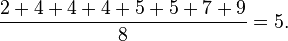
There are eight data points in total, with a mean (or average) value of 5:
To calculate the standard deviation, we compute the difference of each data point from the mean, and square the result:

Next we average these values and take the square root, which gives the standard deviation:

Therefore, the population above has a standard deviation of 2.
Note that we are assuming that we are dealing with a complete population. If our 8 values are obtained by random sampling from some parent population, we might prefer to compute the sample standard deviation using a denominator of 7 instead of 8. See below for an explanation.
[edit] Definition
[edit] Probability distribution or random variable
Let X be a random variable with mean value μ:
![E[X] = \mu\,\!](http://upload.wikimedia.org/math/8/4/3/84316e6eccfe860c66723f4598d0d700.png)
Here E denotes the average or expected value of X. Then the standard deviation of X is the quantity
![\sigma = \sqrt{E\left[(X - \mu)^2\right]}.](http://upload.wikimedia.org/math/7/c/8/7c89b6610aa146e7ef514bc3edcd0471.png)
That is, the standard deviation σ is the square root of the average value of (X – μ)2.
In the case where X takes random values from a finite data set  , with each value having the same probability, the standard deviation is

or, using summation notation,

The standard deviation of a (univariate) probability distribution is the same as that of a random variable having that distribution. Not all random variables have a standard deviation, since these expected values need not exist. For example, the standard deviation of a random variable which follows a Cauchy distribution is undefined because its E(X) is undefined.
[edit] Continuous random variable
Continuous distributions usually give a formula for calculating the standard deviation as a function of the parameters of the distribution. In general, the standard deviation of a continuous real-valued random variable X with probability density function p(x) is

where
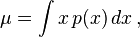
and where the integrals are definite integrals taken for x ranging over the range of X.
[edit] Discrete random variable or data set
The standard deviation of a discrete random variable is the root-mean-square (RMS) deviation of its values from the mean.
If the random variable X takes on N values  (which are real numbers) with equal probability, then its standard deviation σ can be calculated as follows:
- Find the mean,
 , of the values.
 - For each value xi calculate its deviation (
 ) from the mean.
 - Calculate the squares of these deviations.
- Find the mean of the squared deviations. This quantity is the variance σ2.
- Take the square root of the variance.
This calculation is described by the following formula:

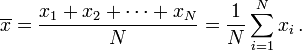
where is the arithmetic mean of the values xi, defined as:
If not all values have equal probability, but the probability of value xi equals pi, the standard deviation can be computed by:
 and
and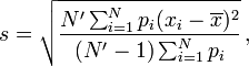
where

and N' is the number of non-zero weight elements.
The standard deviation of a data set is the same as that of a discrete random variable that can assume precisely the values from the data set, where the point mass for each value is proportional to its multiplicity in the data set.
[edit] Example
Suppose we wished to find the standard deviation of the data set consisting of the values 3, 7, 7, and 19.
Step 1: find the arithmetic mean (average) of 3, 7, 7, and 19,

Step 2: find the deviation of each number from the mean,

Step 3: square each of the deviations, which amplifies large deviations and makes negative values positive,

Step 4: find the mean of those squared deviations,

Step 5: take the non-negative square root of the quotient (converting squared units back to regular units),

So, the standard deviation of the set is 6. This example also shows that, in general, the standard deviation is different from the mean absolute deviation (which is 5 in this example).
Note that if the above data set represented only a sample from a greater population, a modified standard deviation would be calculated (explained below) to estimate the population standard deviation, which would give 6.93 for this example.
[edit] Simplification of the formula
The calculation of the sum of squared deviations can be simplified as follows:

Applying this to the original formula for standard deviation gives:
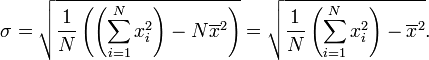
This can be memorized as taking the square root of (the average of the squares less the square of the average).
[edit] Estimating population standard deviation from sample standard deviation
In the real world, finding the standard deviation of an entire population is unrealistic except in certain cases, such as standardized testing, where every member of a population is sampled. In most cases, the standard deviation is estimated by examining a random sample taken from the population. Using the definition given above for a data set and applying it to a small or moderately-sized sample results in an estimate that tends to be too low: it is a biased estimator. The most common measure used is an adjusted version, the sample standard deviation, which is defined by

where  is the sample and is the mean of the sample. This correction (the use of N − 1 instead of N) is known as Bessel's correction. Note that by definition of standard deviation, the "standard deviation of the sample" uses N, while the term "sample standard deviation" is used for the corrected estimator (using N − 1). The denominator N − 1 can be understood intuitively as the number of degrees of freedom in the vector of residuals,
  .
.
The reason for this definition is that s2 is an unbiased estimator for the variance σ2 of the underlying population, if that variance exists and the sample values are drawn independently with replacement. However, s is not an unbiased estimator for the standard deviation σ; it tends to underestimate the population standard deviation. Although an unbiased estimator for σ is known when the random variable is normally distributed, the formula is complicated and amounts to a minor correction: see Unbiased estimation of standard deviation. Moreover, unbiasedness, in this sense of the word, is not always desirable; see bias of an estimator.
Another estimator sometimes used is the similar, uncorrected expression, the "standard deviation of the sample":

This form has a uniformly smaller mean squared error than does the unbiased estimator, and is the maximum-likelihood estimate when the population is normally distributed.
[edit] Properties of standard deviation
For constant c and random variables X and Y:


where  and
and  stand for variance and covariance, respectively.
[edit] Interpretation and application
A large standard deviation indicates that the data points are far from the mean and a small standard deviation indicates that they are clustered closely around the mean.
For example, each of the three populations {0, 0, 14, 14}, {0, 6, 8, 14} and {6, 6, 8, 8} has a mean of 7. Their standard deviations are 7, 5, and 1, respectively. The third population has a much smaller standard deviation than the other two because its values are all close to 7. In a loose sense, the standard deviation tells us how far from the mean the data points tend to be. It will have the same units as the data points themselves. If, for instance, the data set {0, 6, 8, 14} represents the ages of a population of four siblings in years, the standard deviation is 5 years.
As another example, the population {1000, 1006, 1008, 1014} may represent the distances traveled by four athletes, measured in meters. It has a mean of 1007 meters, and a standard deviation of 5 meters.
Standard deviation may serve as a measure of uncertainty. In physical science for example, the reported standard deviation of a group of repeated measurements should give the precision of those measurements. When deciding whether measurements agree with a theoretical prediction, the standard deviation of those measurements is of crucial importance: if the mean of the measurements is too far away from the prediction (with the distance measured in standard deviations), then the theory being tested probably needs to be revised. This makes sense since they fall outside the range of values that could reasonably be expected to occur if the prediction were correct and the standard deviation appropriately quantified. See prediction interval.
[edit] Application examples
The practical value of understanding the standard deviation of a set of values is in appreciating how much variation there is from the "average" (mean).
[edit] Weather
As a simple example, consider average temperatures for cities. While two cities may each have an average temperature of 15 °C, it's helpful to understand that the range for cities near the coast is smaller than for cities inland, which clarifies that, while the average is similar, the chance for variation is greater inland than near the coast.
So, an average of 15 occurs for one city with highs of 25 °C and lows of 5 °C, and also occurs for another city with highs of 18 and lows of 12. The standard deviation allows us to recognize that the average for the city with the wider variation, and thus a higher standard deviation, will not offer as reliable a prediction of temperature as the city with the smaller variation and lower standard deviation.
[edit] Sports
Another way of seeing it is to consider sports teams. In any set of categories, there will be teams that rate highly at some things and poorly at others. Chances are, the teams that lead in the standings will not show such disparity, but will perform well in most categories. The lower the standard deviation of their ratings in each category, the more balanced and consistent they will tend to be. Whereas, teams with a higher standard deviation will be more unpredictable. For example, a team that is consistently bad in most categories will have a low standard deviation. A team that is consistently good in most categories will also have a low standard deviation. However, a team with a high standard deviation might be the type of team that scores a lot (strong offense) but also concedes a lot (weak defense), or, vice versa, that might have a poor offense but compensates by being difficult to score on.
Trying to predict which teams, on any given day, will win, may include looking at the standard deviations of the various team "stats" ratings, in which anomalies can match strengths vs. weaknesses to attempt to understand what factors may prevail as stronger indicators of eventual scoring outcomes.
In racing, a driver is timed on successive laps. A driver with a low standard deviation of lap times is more consistent than a driver with a higher standard deviation. This information can be used to help understand where opportunities might be found to reduce lap times.
[edit] Finance
In finance, standard deviation is a representation of the risk associated with a given security (stocks, bonds, property, etc.), or the risk of a portfolio of securities (actively managed mutual funds, index mutual funds, or ETFs). Risk is an important factor in determining how to efficiently manage a portfolio of investments because it determines the variation in returns on the asset and/or portfolio and gives investors a mathematical basis for investment decisions (known as mean-variance optimization). The overall concept of risk is that as it increases, the expected return on the asset will increase as a result of the risk premium earned – in other words, investors should expect a higher return on an investment when said investment carries a higher level of risk, or uncertainty of that return. When evaluating investments, investors should estimate both the expected return and the uncertainty of future returns. Standard deviation provides a quantified estimate of the uncertainty of future returns.
For example, let's assume an investor had to choose between two stocks. Stock A over the last 20 years had an average return of 10%, with a standard deviation of 20 percentage points (pp) and Stock B, over the same period, had average returns of 12%, but a higher standard deviation of 30 pp. On the basis of risk and return, an investor may decide that Stock A is the safer choice, because Stock B's additional 2% points of return is not worth the additional 10 pp standard deviation (greater risk or uncertainty of the expected return). Stock B is likely to fall short of the initial investment (but also to exceed the initial investment) more often than Stock A under the same circumstances, and is estimated to return only 2% more on average. In this example, Stock A is expected to earn about 10%, plus or minus 20 pp (a range of 30% to -10%), about two-thirds of the future year returns. When considering more extreme possible returns or outcomes in future, an investor should expect results of up to 10% plus or minus 90 pp, or a range from 100% to -80%, which includes outcomes for three standard deviations from the average return (about 99.7% of probable returns).
Calculating the average return (or arithmetic mean) of a security over a given number of periods will generate an expected return on the asset. For each period, subtracting the expected return from the actual return results in the variance. Square the variance in each period to find the effect of the result on the overall risk of the asset. The larger the variance in a period, the greater risk the security carries. Taking the average of the squared variances results in the measurement of overall units of risk associated with the asset. Finding the square root of this variance will result in the standard deviation of the investment tool in question.
[edit] Geometric interpretation
To gain some geometric insights, we will start with a population of three values, x1, x2, x3. This defines a point P = (x1, x2, x3) in R3. Consider the line L = {(r, r, r) : r in R}. This is the "main diagonal" going through the origin. If our three given values were all equal, then the standard deviation would be zero and P would lie on L. So it is not unreasonable to assume that the standard deviation is related to the distance of P to L. And that is indeed the case. Moving orthogonally from P to the line L, one hits the point:

whose coordinates are the mean of the values we started out with. A little algebra shows that the distance between P and R (which is the same as the distance between P and the line L) is given by σ√3. An analogous formula (with 3 replaced by N) is also valid for a population of N values; we then have to work in RN.
[edit] Chebyshev's inequality
An observation is rarely more than a few standard deviations away from the mean. Chebyshev's inequality entails the following bounds for all distributions for which the standard deviation is defined.
- At least 50% of the values are within √2 standard deviations from the mean.
- At least 75% of the values are within 2 standard deviations from the mean.
- At least 89% of the values are within 3 standard deviations from the mean.
- At least 94% of the values are within 4 standard deviations from the mean.
- At least 96% of the values are within 5 standard deviations from the mean.
- At least 97% of the values are within 6 standard deviations from the mean.
- At least 98% of the values are within 7 standard deviations from the mean.
And in general:
- At least (1 − 1/k2) × 100% of the values are within k standard deviations from the mean.
[edit] Rules for normally distributed data
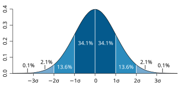
The central limit theorem says that the distribution of a sum of many independent, identically distributed random variables tends towards the normal distribution. If a data distribution is approximately normal then about 68% of the values are within 1 standard deviation of the mean (mathematically, μ ± σ, where μ is the arithmetic mean), about 95% of the values are within two standard deviations (μ ± 2σ), and about 99.7% lie within 3 standard deviations (μ ± 3σ). This is known as the 68-95-99.7 rule, or the empirical rule.
For various values of z, the percentage of values expected to lie in the symmetric confidence interval (−zσ,zσ) are as follows:
| zσ | percentage |
|---|---|
| 1σ | 68.2689492% |
| 1.645σ | 90% |
| 1.960σ | 95% |
| 2σ | 95.4499736% |
| 2.576σ | 99% |
| 3σ | 99.7300204% |
| 3.2906σ | 99.9% |
| 4σ | 99.993666% |
| 5σ | 99.99994267% |
| 6σ | 99.9999998027% |
| 7σ | 99.9999999997440% |
[edit] Relationship between standard deviation and mean
The mean and the standard deviation of a set of data are usually reported together. In a certain sense, the standard deviation is a "natural" measure of statistical dispersion if the center of the data is measured about the mean. This is because the standard deviation from the mean is smaller than from any other point. The precise statement is the following: suppose x1, ..., xn are real numbers and define the function:

Using calculus, or simply by completing the square, it is possible to show that σ(r) has a unique minimum at the mean:

The coefficient of variation of a sample is the ratio of the standard deviation to the mean. It is a dimensionless number that can be used to compare the amount of variance between populations with different means.
If we want to obtain the mean by sampling the distribution then the standard deviation of the mean is related to the standard deviation of the distribution by:
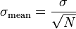
where N is the number of samples used to sample the mean.
[edit] Rapid calculation methods
The following two formulas are a useful representation of running (continuous) standard deviation. A set of three power sums s0,1,2 are each computed over a set of N values of x, denoted as xk.

Note that s0 raises x to the zero power, and since x0 is always 1, s0 evaluates to N.
Given the results of these three running sumations, one can use s0,1,2 at any time to compute the current value of the running standard deviation. This crafty definition for sj allows us to easily represent the two different phases (summation computation sj, and σ calculation).
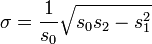
Similarly for sample standard deviation,

In a computer implementation, as the three sj sums become large, we need to consider round-off error, arithmetic overflow, and arithmetic underflow. Below is a better method for calculating running sums method with reduced rounding errors:
- A1 = x1

where A is the mean value.
- Q1 = 0

sample variance:

standard variance

For weighted distribution it is somewhat more complicated: The mean is given by:
- A1 = x1

where wj are the weights.
- Q1 = 0


where n is the total number of elements, and n' is the number of elements with non-zero weights. The above formulas become equal to the simpler formulas given above if we take all weights equal to 1.
[edit] See also
|
[edit] References
- ^ Dodge, Y. (2003) The Oxford Dictionary of Statistical Terms, OUP, ISBN 0-19-920613-9
- ^ Pearson, K. (1894) On the dissection of asymmetrical frequency curves. Phil. Trans. Roy. Soc. London, A, 185, 719–810
- ^ http://jeff560.tripod.com/mathword.html Earliest Known Uses of Some of the Words of Mathematics
[edit] External links
- A Guide to Understanding & Calculating Standard Deviation
- Interactive Demonstration and Standard Deviation Calculator
- Standard Deviation - an explanation without maths
- Standard Deviation, an elementary introduction
- Standard Deviation, a simpler explanation for writers and journalists
- Standard Deviation Calculator
- Texas A&M Standard Deviation and Confidence Interval Calculators
|
|||||||||||||||||||||||||||||||||||||||||||||||||||||||||

