Convolution

From Wikipedia, the free encyclopedia

For the usage in formal language theory, see Convolution (computer science).

Visual explanation of convolution.
1.Express each function in terms of a dummy variable

τ.

2.Transpose one of the functions:

g (τ)

→

g ( - τ).

3.Add a time-offset, t, which allows

g (t - τ)

to slide along the

τ

-axis.
4.Start t at -∞ and slide it all the way to +∞. Wherever the two functions intersect, find the integral of their product. In other words, compute a sliding, weighted-average of function

f (τ)

, where the weighting function is

g ( - τ).

The resulting waveform (not shown here) is the convolution of functions f and g. If f(t) is a unit impulse, the result of this process is simply g(t), which is therefore called the impulse response.

In mathematics and, in particular, functional analysis, convolution is a mathematical operation on two functions f and g, producing a third function that is typically viewed as a modified version of one of the original functions. Convolution is similar to cross-correlation. It has applications that include statistics, computer vision, image and signal processing, electrical engineering, and differential equations.

The convolution can be defined for functions on groups other than Euclidean space. In particular, the circular convolution can be defined for periodic functions (that is, functions on the circle), and the discrete convolution can be defined for functions on the set of integers. These generalizations of the convolution have applications in the field of numerical analysis and numerical linear algebra, and in the design and implementation of finite impulse response filters in signal processing.

[edit] Definition

The convolution of ƒ and g is written ƒ∗g. It is defined as the integral of the product of the two functions after one is reversed and shifted. As such, it is a particular kind of integral transform:

$(f * g )(t)\ \ \,$	$\stackrel{\mathrm{def}}{=}\ \int_{-\infty}^{\infty} f(\tau)\cdot g(t - \tau)\, d\tau$
	$= \int_{-\infty}^{\infty} f(t-\tau)\cdot g(\tau)\, d\tau.$ (commutativity)

While the symbol t is used above, it need not represent the time domain. But in that context, the convolution formula can be described as a weighted average of the function ƒ(τ) at the moment t where the weighting is given by g(−τ) simply shifted by amount t. As t changes, the weighting function emphasizes different parts of the input function.

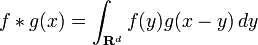
More generally, if f and g are complex-valued functions on R^d, then their convolution may be defined as the integral:

$(f * g )(x) = \int_{\mathbf{R}^d} f(y)g(x-y)\,dy = \int_{\mathbf{R}^d} f(x-y)g(y)\,dy.$

[edit] Circular convolution

Main article: Circular convolution

When a function g_T is periodic, with period T, then for functions, ƒ, such that ƒ∗g_T exists, the convolution is also periodic and identical to:

$(f * g_T)(t) \equiv \int_{t_0}^{t_0+T} \left[\sum_{k=-\infty}^{\infty} f(\tau + kT)\right] g_T(t - \tau)\ d\tau,\,$

where t_o is an arbitrary choice. The summation is called a periodic extension of the function ƒ.

If g_T is a periodic extension of another function, g, then ƒ∗g_T is known as a circular, cyclic, or periodic convolution of ƒ and g.

[edit] Discrete convolution

For complex-valued functions ƒ, g defined on the set of integers, the discrete convolution of ƒ and g is given by:

$(f * g)[n]\ \stackrel{\mathrm{def}}{=}\ \sum_{m=-\infty}^{\infty} f[m]\cdot g[n - m]\,$

$= \sum_{m=-\infty}^{\infty} f[n-m]\cdot g[m].\,$ (commutativity)

When multiplying two polynomials, the coefficients of the product are given by the convolution of the original coefficient sequences, extended with zeros where necessary to avoid undefined terms; this is known as the Cauchy product of the coefficients of the two polynomials.

[edit] Circular discrete convolution

When a function g_N is periodic, with period N, then for functions, ƒ, such that ƒ∗g_N exists, the convolution is also periodic and identical to:

$(f * g_N)[n] \equiv \sum_{m=0}^{N-1} \left(\sum_{k=-\infty}^{\infty} {f}[m+kN] \right) g_N[n-m].\,$

The summation on k is called a periodic extension of the function ƒ.

If g_N is a periodic extension of another function, g, then ƒ∗g_N is known as a circular, cyclic, or periodic convolution of ƒ and g.

When the non-zero durations of both ƒ and g are limited to the interval [0, N-1], ƒ∗g_N reduces to these common forms:

$(f * g_N)[n] = \sum_{m=0}^{N-1} f[m]\ g_N[n-m]\,$

(Eq.1)

$= \sum_{m=0}^n f[m]\ g[n-m] + \sum_{m=n+1}^{N-1} f[m]\ g[N+n-m]\,$

$= \sum_{m=0}^{N-1} f[m]\ g[(n-m)_{\mod{N}}]\quad \stackrel{\mathrm{def}}{=}\quad (f *_N g)[n].\,$

The notation $(f *_N g)\,$ for cyclic convolution denotes convolution over the cyclic group of integers modulo N.

[edit] Fast convolution algorithms

In many situations, discrete convolutions can be converted to circular convolutions so that fast transforms with a convolution property can be used to implement the computation. For example, convolution of digit sequences is the kernel operation in multiplication of multi-digit numbers, which can therefore be efficiently implemented with transform techniques (Knuth 1997, §4.3.3.C; von zur Gathen & Gerhard 2003, §8.2).

Eq.1 requires N arithmetic operations per output value and N² operations for N outputs. That can be significantly reduced with any of several fast algorithms. Digital signal processing and other applications typically use fast convolution algorithms to reduce the cost of the convolution to O(N log N) complexity.

The most common fast convolution algorithms use fast Fourier transform (FFT) algorithms via the circular convolution theorem. Specifically, the circular convolution of two finite-length sequences is found by taking an FFT of each sequence, multiplying pointwise, and then performing an inverse FFT. Convolutions of the type defined above are then efficiently implemented using that technique in conjunction with zero-extension and/or discarding portions of the output. Other fast convolution algorithms, such as the Schönhage-Strassen algorithm, use fast Fourier transforms in other rings.

[edit] Domain of definition

The convolution of two complex-valued functions on R^d

$f*g(x) = \int_{\mathbf{R}^d}f(y)g(x-y)\,dy$

is well-defined only if ƒ and g decay sufficiently rapidly at infinity in order for the integral to exist. Conditions for the existence of the convolution may be tricky, since a blow-up in g at infinity can be easily offset by sufficiently rapid decay in ƒ. The question of existence thus may involve different conditions on ƒ and g.

[edit] Compactly supported functions

If ƒ and g are compactly supported continuous functions, then their convolution exists, and is also compactly supported and continuous (Hörmander). More generally, if either function (say ƒ) is compactly supported and the other is locally integrable, then the convolution ƒ∗g is well-defined and continuous.

[edit] Integrable functions

The convolution of ƒ and g exists if ƒ and g are both Lebesgue integrable functions (in L¹(R^d)), and ƒ∗g is also integrable (Stein & Weiss 1971, Theorem 1.3). This is a consequence of Tonelli's theorem. Likewise, if ƒ∈L¹(R^d) and g ∈ L^p(R^d) where 1 ≤ p ≤ ∞, then ƒ∗g ∈ L^p(R^d) and

$\|{f}*g\|_p\le \|f\|_1\|g\|_p.$

[edit] Functions of rapid decay

In addition to compactly supported functions and integrable functions, functions that have sufficiently rapid decay at infinity can also be convolved. An important feature of the convolution is that if ƒ and g both decay rapidly, then ƒ∗g also decays rapidly. In particular, if ƒ and g are rapidly decreasing functions, then so is the convolution ƒ∗g. Combined with the fact that convolution commutes with differentiation (see Properties), it follows that the class of Schwartz functions is closed under convolution.

[edit] Distributions

Main article: Distribution (mathematics)

Under some circumstances, it is possible to define the convolution of a function with a distribution, or of two distributions. If ƒ is a compactly supported function and g is a distribution, then ƒ∗g is a smooth function defined by a distributional formula analogous to

$\int_{\mathbf{R}^d} {f}(y)g(x-y)\,dy.$

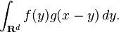
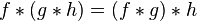
More generally, it is possible to extend the definition of the convolution in a unique way so that the associative law

$f*(g*\phi) = (f*g)*\phi\,$

remains valid in the case where ƒ is a distribution, and g a compactly supported distribution (Hörmander 1983, §4.2).

[edit] Properties

[edit] Algebraic properties

[edit] Differentiation

In the one variable case,

$\frac{d}{dx}({f} * g) = \frac{df}{dx} * g = {f} * \frac{dg}{dx} \,$

where d /dx is the derivative. More generally, in the case of functions of several variables, an analogous formula holds with the partial derivative:

$\frac{\partial}{\partial x_i}({f} * g)(x) = \frac{\partial f}{\partial x_i} * g = {f} * \frac{\partial g}{\partial x_i}.$

A particular consequence of this is that the convolution can be viewed as a "smoothing" operation: the convolution of ƒ and g is differentiable as many times as ƒ and g are together.

In the discrete case, the difference operator D ƒ(n) = ƒ(n+1) − ƒ(n) satisfies an analogous relationship:

$D(f*g) = (Df)*g = f*(Dg).\,$

[edit] Convolution theorem

The convolution theorem states that

$\mathcal{F}\{f * g\} = k\cdot \mathcal{F}\{f\}\cdot \mathcal{F}\{g\}$

where $\mathcal{F}\{f\}\,$ denotes the Fourier transform of $f$ , and $k$ is a constant that depends on the specific normalization of the Fourier transform (see “Properties of the fourier transform”). Versions of this theorem also hold for the Laplace transform, two-sided Laplace transform, Z-transform and Mellin transform.

See also the less trivial Titchmarsh convolution theorem.

[edit] Translation invariance

The convolution commutes with translations, meaning that

$\tau_x ({f}*g) = (\tau_x f)*g = {f}*(\tau_x g)\,$

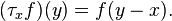
where τ_xƒ is the translation of the function ƒ by x defined by

$(\tau_x f)(y) = f(y-x).\,$

Furthermore, under certain conditions, convolution is the most general translation invariant operation. Roughly speaking, the following holds

Suppose that S is a linear operator acting on functions which commutes with translations: S(τ_xƒ) = τ_x(Sƒ) for all x. Then S is given as convolution with a function (or distribution) g_S; that is Sƒ = g_S∗ƒ.

Thus any translation invariant operation can be represented as a convolution. Convolutions play an important role in the study of time-invariant systems, and especially LTI system theory. The representing function g_S is the impulse response of the transformation S.

[edit] Convolution inverse

Main article: Convolution power#Convolution inverse

Many functions have an inverse element, f^(-1), which satisfies the relationship:

$f^{(-1)} * f = \delta. \,$

These functions form an abelian group, with the group operation being convolution.

[edit] Convolutions on groups

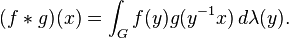
If G is a suitable group endowed with a measure λ (for instance, a locally compact Hausdorff topological group with the Haar measure) and if f and g are real or complex valued integrable functions on G, then we can define their convolution by

$(f * g)(x) = \int_G f(y) g(y^{-1}x)\,d\lambda(y). \,$

In the case when λ is the Haar integral and G is not unimodular, this is not the same as $\int f(xy^{-1})g(y)d\lambda(y)$ . The choice between the two is such that it coincides with the convolution of measures (see below).

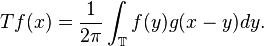
The circle group T with the Lebesgue measure is an immediate example. For a fixed g in L¹(T), we have the following familiar operator acting on the Hilbert space L²(T):

$T {f}(x) = \frac{1}{2 \pi} \int_{\mathbb{T}} {f}(y) g( x - y) dy.$

The operator T is compact. A direct calculation shows that its adjoint T* is convolution with

$\bar{g}(-y).$

By the commutativity property cited above, T is normal, i.e. T*T = TT*. Also, T commutes with the translation operators. Consider the family S of operators consisting of all such convolutions and the translation operators. S is a commuting family of normal operators. According to spectral theory, there exists an orthonormal basis {h_k} that simultaneously diagonalizes S. This characterizes convolutions on the circle. Specifically, we have

$h_k (x) = e^{ikx},\;$

which are precisely the characters of T. Each convolution is a compact multiplication operator in this basis. This can be viewed as a version of the convolution theorem discussed above.

An even simpler discrete example is a finite cyclic group of order n, where convolution operators are represented by circulant matrices, and can be diagonalized by the discrete Fourier transform.

The above example may convince one that convolutions arise naturally in the context of harmonic analysis on groups. For more general groups, it is also possible to give, for instance, a Convolution Theorem, however it is much more difficult to phrase and requires representation theory for these types of groups and the Peter-Weyl theorem. It is very difficult to do these calculations without more structure, and Lie groups turn out to be the setting in which these things are done.^{[clarification needed]}

[edit] Convolution of measures

Let G be a topological group. If μ and ν are Borel measures on G, then their convolution μ∗ν is defined by

$(\mu * \nu)(E) = \int\!\!\!\int 1_E(xy) \,d\mu(x) \,d\nu(y)$

for each measurable subset E of G.

In the case when G is locally compact with (left-)Haar measure λ, and μ and ν are absolutely continuous with respect to a λ, so that each has a density function, then the convolution μ∗ν is also absolutely continuous, and its density function is just the convolution of the two separate density functions.

If μ and ν are probability measures, then the convolution μ∗ν is the probability distribution of the sum X + Y of two independent random variables X and Y whose respective distributions are μ and ν.

[edit] Applications

Convolution and related operations are found in many applications of engineering and mathematics.

In electrical engineering and digital signal processing, the convolution of one function (the input) with a second function (the impulse response) gives the output of a linear time-invariant system (LTI). At any given moment, the output is an accumulated effect of all the prior values of the input function, with the most recent values typically having the most influence (expressed as a multiplicative factor). The impulse response function provides that factor as a function of the elapsed time since each input value occurred.
- Convolution amplifies or attenuates each frequency component of the input independently of the other components.
In statistics, as noted above, a weighted moving average is a convolution.
In probability theory, the probability distribution of the sum of two independent random variables is the convolution of their individual distributions.
In optics, many kinds of "blur" are described by convolutions. A shadow (e.g. the shadow on the table when you hold your hand between the table and a light source) is the convolution of the shape of the light source that is casting the shadow and the object whose shadow is being cast. An out-of-focus photograph is the convolution of the sharp image with the shape of the iris diaphragm. The photographic term for this is bokeh.
Similarly, in digital image processing, convolutional filtering plays an important role in many important algorithms in edge detection and related processes.
In linear acoustics, an echo is the convolution of the original sound with a function representing the various objects that are reflecting it.
In artificial reverberation (digital signal processing, pro audio), convolution is used to map the impulse response of a real room on a digital audio signal (see previous and next point for additional information).
In time-resolved fluorescence spectroscopy, the excitation signal can be treated as a chain of delta pulses, and the measured fluorescence is a sum of exponential decays from each delta pulse.
In physics, wherever there is a linear system with a "superposition principle", a convolution operation makes an appearance.
This is the fundamental problem term in the Navier–Stokes equations relating to the Clay Mathematics Millennium Problem and the associated million dollar prize.

[edit] See also

LTI system theory#Impulse response and convolution
Toeplitz matrix (convolutions can be considered a Toeplitz matrix operation where each row is a shifted copy of the convolution kernel)
- Circulant matrix
Cross-correlation
Deconvolution
Dirichlet convolution
Titchmarsh convolution theorem
Convolution power
Analog signal processing
List of convolutions of probability distributions
Jan Mikusinski

[edit] References

Bracewell, R. (1986), The Fourier Transform and Its Applications (2nd ed ed.), McGraw-Hill .
Hörmander, L. (1983), The analysis of linear partial differential operators I, Grundl. Math. Wissenschaft., 256, Springer, MR 0717035, ISBN 3-540-12104-8 .
Knuth, Donald (1997), Seminumerical Algorithms (3rd. ed.), Reading, Massachusetts: Addison-Wesley, ISBN 0-201-89684-2 .
Sobolev, V.I. (2001), "Convolution of functions", in Hazewinkel, Michiel, Encyclopaedia of Mathematics, Kluwer Academic Publishers, ISBN 978-1556080104 .
Stein, Elias; Weiss, Guido (1971), Introduction to Fourier Analysis on Euclidean Spaces, Princeton University Press, ISBN 0-691-08078-X .
Strichartz, R. (1994), A Guide to Distribution Theory and Fourier Transforms, CRC Press, ISBN 0849382734 .
Titchmarsh, E (1948), Introduction to the theory of Fourier integrals (2nd ed.) (published 1986), ISBN 978-0828403245 .
Treves, François (1967), Topological Vector Spaces, Distributions and Kernels, Academic Press .
von zur Gathen, J.; Gerhard, J. (2003), Modern Computer Algebra, Cambridge University Press, ISBN 0-521-82646-2 .

[edit] External links

Wikimedia Commons has media related to: Convolution

http://www.nitte.ac.in/downloads/Conv-LTI.pdf
Convolution, on The Data Analysis BriefBook
http://www.jhu.edu/~signals/convolve/index.html Visual convolution Java Applet.
http://www.jhu.edu/~signals/discreteconv2/index.html Visual convolution Java Applet for Discrete Time functions.
Lectures on Image Processing: A collection of 18 lectures in pdf format from Vanderbilt University. Lecture 7 is on 2-D convolution., by Alan Peters.
- http://www.vuse.vanderbilt.edu/~rap2/EECE253/EECE253_01_Intro.pdf
Convolution Kernel Mask Operation Interactive tutorial
Convolution at MathWorld