Odds ratio

From Wikipedia, the free encyclopedia

The odds ratio is a measure of effect size, describing the strength of association or non-independence between two binary data values. It is used as a descriptive statistic, and plays an important role in logistic regression.

[edit] Definition

[edit] Definition in terms of group-wise odds

The odds ratio is the ratio of the odds of an event occurring in one group to the odds of it occurring in another group, or to a sample-based estimate of that ratio. These groups might be men and women, an experimental group and a control group, or any other dichotomous classification. If the probabilities of the event in each of the groups are p₁ (first group) and p₂ (second group), then the odds ratio is:

${ p_1/(1-p_1) \over p_2/(1-p_2)}={ p_1/q_1 \over p_2/q_2}=\frac{\;p_1q_2\;}{\;p_2q_1\;},$

where q_x = 1 − p_x. An odds ratio of 1 indicates that the condition or event under study is equally likely in both groups. An odds ratio greater than 1 indicates that the condition or event is more likely in the first group. And an odds ratio less than 1 indicates that the condition or event is less likely in the first group. The odds ratio must be greater than or equal to zero if it is defined. It is undefined if p₂q₁ equals zero.

[edit] Definition in terms of joint and conditional probabilities

The odds ratio can also be defined in terms of the joint probability distribution of two binary random variables. The joint distribution of binary random variables X and Y can be written

	Y = 1	Y = 0
X = 1	$p 11$	$p 10$
X = 0	$p 01$	$p 00$

where $p 11$ , $p 10$ , $p 01$ and $p 00$ are non-negative "cell probabilities" that sum to one. The odds for Y within the two subpopulations defined by X = 1 and X = 0 are defined in terms of the conditional probabilities given X:

	Y = 1	Y = 0
X = 1	$p 11 / (p 11 + p 10)$	$p 10 / (p 11 + p 10)$
X = 0	$p 01 / (p 01 + p 00)$	$p 00 / (p 01 + p 00)$

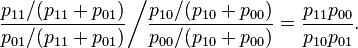
Thus the odds ratio is

${ \dfrac{p_{11}/(p_{11}+p_{10})}{p_{10}/(p_{11}+p_{10})} \bigg / \dfrac{p_{01}/(p_{01}+p_{00})}{p_{00}/(p_{01}+p_{00})}} = \dfrac{p_{11}p_{00}}{p_{10}p_{01}}.$

The simple expression on the right, above, is easy to remember as the product of the probabilities of the "concordant cells" (X = Y) divided by the product of the probabilities of the "discordant cells" (X ≠ Y). However note that in some applications the labeling of categories as zero and one is arbitrary, so there is nothing special about concordant versus discordant values in these applications.

[edit] Symmetry

If we had calculated the odds ratio based on the conditional probabilities given Y,

	Y = 1	Y = 0
X = 1	$p 11 / (p 11 + p 01)$	$p 10 / (p 10 + p 00)$
X = 0	$p 01 / (p 11 + p 01)$	$p 00 / (p 10 + p 00)$

we would have gotten the same result

${ \dfrac{p_{11}/(p_{11}+p_{01})}{p_{01}/(p_{11}+p_{01})} \bigg / \dfrac{p_{10}/(p_{10}+p_{00})}{p_{00}/(p_{10}+p_{00})}} = \dfrac{p_{11}p_{00}}{p_{10}p_{01}}.$

Other measures of effect size for binary data such as the relative risk do not have this symmetry property.

[edit] Relation to statistical independence

If X and Y are independent, their joint probabilities can be expressed in terms of their marginal probabilities $p x = P (X = 1)$ and $p y = P (Y = 1)$ , as follows

	Y = 1	Y = 0
X = 1	$p x p y$	$p x (1 - p y)$
X = 0	$(1 - p x) p y$	$(1 - p x)(1 - p y)$

In this case, the odds ratio equals one, and conversely the odds ratio can only equal one if the joint probabilities can be factored in this way. Thus the odds ratio equals one if and only if X and Y are independent.

[edit] Example

Suppose that in a sample of 100 men, 90 have drunk wine in the previous week, while in a sample of 100 women only 20 have drunk wine in the same period. The odds of a man drinking wine are 90 to 10, or 9:1, while the odds of a woman drinking wine are only 20 to 80, or 1:4 = 0.25:1. The odds ratio is thus 9/0.25, or 36, showing that men are much more likely to drink wine than women. Using the above formula for the calculation yields the same result:

${ 0.9/0.1 \over 0.2/0.8}=\frac{\;0.9\times 0.8\;}{\;0.1\times 0.2\;} ={0.72 \over 0.02} = 36.$

The above example also shows how odds ratios are sometimes sensitive in stating relative positions: in this sample men are 90/20 = 4.5 times more likely to have drunk wine than women, but have 36 times the odds. The logarithm of the odds ratio, the difference of the logits of the probabilities, tempers this effect, and also makes the measure symmetric with respect to the ordering of groups. For example, using natural logarithms, an odds ratio of 36/1 maps to 3.584, and an odds ratio of 1/36 maps to −3.584.

[edit] Statistical inference

Confidence intervals and hypothesis tests relating to odds ratios are constructed in terms of the "log odds ratio," which is the natural logarithm of the odds ratio. If we use the joint probability notation defined above, the population log odds ratio is

${\log\Big(\frac{p_{11}p_{00}}{p_{01}p_{10}}\Big) = \log\big(p_{11}) + \log(p_{00}\big) - \log(p_{10}) - \log(p_{01})}.\,$

If we observe data in the form of a contingency table

	Y = 1	Y = 0
X = 1	$n 11$	$n 10$
X = 0	$n 01$	$n 00$

then the probabilities in the joint distribution can be estimated as

	Y = 1	Y = 0
X = 1	$\hat{p}_{11}$	$\hat{p}_{10}$
X = 0	$\hat{p}_{01}$	$\hat{p}_{00}$

where $\hat{p}_{ij} = n_{ij}/n$ , with $n = n 11 + n 10 + n 01 + n 00$ being the sum of all four cell counts. The sample log odds ratio is

${L=\log\Bigg(\dfrac{\hat{p}_{11}\hat{p}_{00}}{\hat{p}_{10}\hat{p}_{01}}\Bigg) = \log\Bigg(\dfrac{n_{11}n_{00}}{n_{10}n_{01}}\Bigg)}$ .

The standard error for the log odds ratio is approximately

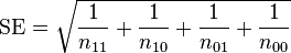${{\rm SE} = \sqrt{\dfrac{1}{n_{11}} + \dfrac{1}{n_{10}} + \dfrac{1}{n_{01}} + \dfrac{1}{n_{00}}}}$ .

This is an asymptotic approximation, and will not give a meaningful result if any of the cell counts are very small. If $L$ is the sample log odds ratio, an approximate 95% confidence interval for the population log odds ratio is $L\pm 2{\rm SE}$ . This can be mapped to $\exp(L-2{\rm SE}),\;\exp(L+2{\rm SE})$ to obtain a 95% confidence interval for the odds ratio. If we wish to test the hypothesis that the population odds ratio equals one, the two-sided p-value is $2 P (Z < - | L | / SE)$ , where $P$ denotes a probability, and $Z$ denotes a standard normal random variable.

[edit] Role in logistic regression

Logistic regression is one way to generalize the odds ratio beyond two binary variables. Suppose we have a binary response variable Y and a binary predictor variable X, and in addition we have other predictor variables Z₁, ..., Z_p that may or may not be binary. If we use multiple logistic regression to regress Y on X, Z₁, ..., Z_p, then the estimated coefficient $\hat{\beta}_x$ for X is related to a conditional odds ratio. Specifically, at the population level

$\exp(\beta_x) = \frac{P(Y=1|X=1, Z_1, \ldots, Z_p)/P(Y=0|X=1, Z_1, \ldots, Z_p)}{P(Y=1|X=0, Z_1, \ldots, Z_p)/P(Y=0|X=0, Z_1, \ldots, Z_p)},$

so $\exp(\hat{\beta}_x)$ is an estimate of this conditional odds ratio. The interpretation of $\exp(\hat{\beta}_x)$ is as an estimate of the odds ratio between Y and X when the values of Z₁, ..., Z_p are held fixed.

[edit] Use in quantitative research

Due to the widespread use of logistic regression in medical and social science research, the odds ratio is commonly used as a means of expressing the results in some forms of clinical trials, in survey research, and in epidemiology, such as in case-control studies. It is often abbreviated "OR" in reports. When data from multiple surveys is combined, it will often be expressed as "pooled OR". The odds ratio, while in itself difficult to interpret, is in such cases used as an estimate of the relative risk. This, however, is only valid when dealing with low-probability events: The formula for the odds is defined as p / (1 − p), so when p moves towards zero, (1 − p) moves towards 1, meaning that as p approaches zero, the odds approaches the risk, and the odds ratio approaches the relative risk.

[edit] Worked example

	Experimental group (E)	Control group (C)	Total
Events (E)	EE or "A" = 15	CE or "B" = 100	115
Non-events (N)	EN or "C" = 135	CN or "D" = 150	285
Total subjects (S)	ES = 150	CS = 250	400
Event rate (ER)	EER = EE / ES = 0.1, or 10%	CER = CE / CS = 0.4, or 40%

Abbreviation	Variable	Equation	Value
ARR	absolute risk reduction (or increase)	= EER − CER	-0.3, or -30%
RRR	relative risk reduction (or increase)	= \|(EER − CER)\| / CER^[1]	0.75
NNT	number needed to treat/number needed to harm	= 1 / ARR	3.33
RR	relative risk	= EER / CER or = (EE / ES) / (CE / CS)	0.25
OR	odds ratio	= (EE / EN) / (CE / CN)	0.167

[edit] See also

[edit] External links

[edit] References

^ Center for Evidence-Based Medicine, University of Toronto (03. April 2007 21:51:20). "Glossary of EBM Terms". University of Toronto. http://www.cebm.utoronto.ca/glossary/index.htm#t. Retrieved on 20.1.2009.

[0] Center for Evidence-Based Medicine, University of Toronto (03. April 2007 21:51:20). "Glossary of EBM Terms". University of Toronto. http://www.cebm.utoronto.ca/glossary/index.htm#t. Retrieved on 20.1.2009.

[1]

Odds ratio

From Wikipedia, the free encyclopedia

Contents

[edit] Definition

[edit] Definition in terms of group-wise odds

[edit] Definition in terms of joint and conditional probabilities

[edit] Symmetry

[edit] Relation to statistical independence

[edit] Example

[edit] Statistical inference

[edit] Role in logistic regression

[edit] Use in quantitative research

[edit] Worked example

[edit] See also

[edit] External links

[edit] References

Views

Personal tools

Navigation

Search

Interaction

Toolbox

Languages