Pearson product-moment correlation coefficient
From Wikipedia, the free encyclopedia
|
|
This article may require cleanup to meet Wikipedia's quality standards. Please improve this article if you can. (January 2008) |
In statistics, the Pearson product-moment correlation coefficient (sometimes referred to as the MCV or PMCC, and typically denoted by r) is a common measure of the correlation (linear dependence) between two variables X and Y. It is very widely used in the sciences as a measure of the strength of linear dependence between two variables, giving a value somewhere between +1 and -1 inclusive. It was first introduced by Francis Galton in the 1880s, and named after Karl Pearson.[1]
In accordance with the usual convention, when calculated for an entire population, the Pearson product-moment correlation is typically designated by the analogous Greek letter, which in this case is ρ (rho). Hence its designation by the Latin letter r implies that it has been computed for a sample (to provide an estimate for that of the underlying population). For these reasons, it is sometimes called "Pearson's r."
Contents |
[edit] Definition
The statistic is defined as the sum of the products of the standard scores of the two measures divided by the degrees of freedom.[2] If the data comes from a sample, then
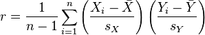
where

are the standard score, sample mean, and sample standard deviation (calculated using n − 1 in the denominator).[2]
If the data comes from a population, then

where

are the standard score, population mean, and population standard deviation (calculated using n in the denominator).
The result obtained is equivalent to dividing the covariance between the two variables by the product of their standard deviations.

[edit] Interpretation
The coefficient ranges from −1 to 1. A value of 1 shows that a linear equation describes the relationship perfectly and positively, with all data points lying on the same line and with Y increasing with X. A score of −1 shows that all data points lie on a single line but that Y increases as X decreases. A value of 0 shows that a linear model is not needed – that there is no linear relationship between the variables.[2]
The linear equation that best describes the relationship between X and Y can be found by linear regression. This equation can be used to "predict" the value of one measurement from knowledge of the other. That is, for each value of X the equation calculates a value which is the best estimate of the values of Y corresponding the specific value. We denote this predicted variable by Y'.
Any value of Y can therefore be defined as the sum of Y′ and the difference between Y and Y′:
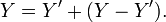
The variance of Y is equal to the sum of the variance of the two components of Y:

Since the coefficient of determination implies that sy.x2 = sy2(1 − r2) we can derive the identity

The square of r is conventionally used as a measure of the association between X and Y. For example, if r2 is 0.90, then 90% of the variance of Y can be "accounted for" by changes in X and the linear relationship between X and Y.[2]
[edit] Gaussianity
The use of mean and standard deviation in the calculation above might suggest that the use of the coefficient requires one to assume that X and Y are normally distributed. The coefficient is fully defined without reference to such assumptions, and it has widespread practical use with the assumption being made[1]. However, if X and Y are assumed to have a bivariate normal distribution certain theoretical results can be derived. Possibly the most useful of these are the formula for the asymptotic (large sample size) variance of the estimated correlation coefficient. Other formulae relate to the probability distribution of the sample estimate and approximations for this.
[edit] See also
- Linear correlation (wikiversity)
- Spearman's rank correlation coefficient
[edit] References
- ^ a b J. L. Rodgers and W. A. Nicewander. Thirteen ways to look at the correlation coefficient. The American Statistician, 42(1):59–66, Feb 1988.
- ^ a b c d Moore, David (August 2006). "4". Basic Practice of Statistics (4 ed.). WH Freeman Company. pp. 90–114. ISBN 0-7167-7463-1.
|
|||||||||||||||||||||||||||||||||||||||||||||||||||||||||

