Polynomial interpolation

From Wikipedia, the free encyclopedia

In the mathematical subfield of numerical analysis, polynomial interpolation is the interpolation of a given data set by a polynomial. In other words, given some data points (such as obtained by sampling), the aim is to find a polynomial which goes exactly through these points.

[edit] Applications

Polynomials can be used to approximate more complicated curves, for example, the shapes of letters in typography, given a few points. A related application is the evaluation of the natural logarithm and trigonometric functions: pick a few known data points, create a lookup table, and interpolate between those data points. This results in significantly faster computations. Polynomial interpolation also forms the basis for algorithms in numerical quadrature and numerical ordinary differential equations.

Polynomial interpolation is also essential to perform sub-quadratic multiplication and squaring such as Karatsuba multiplication and Toom–Cook multiplication, where an interpolation through points on a polynomial which defines the product yields the product itself. For example, given a = f(x) = a₀x⁰ + a₁x¹ + ... and b = g(x) = b₀x⁰ + b₁x¹ + ... then the product ab is equivalent to W(x) = f(x)g(x). Finding points along W(x) by substituting x for small values in f(x) and g(x) yields points on the curve. Interpolation based on those points will yield the terms of W(x) and subsequently the product ab. In the case of Karatsuba multiplication this technique is substantially faster than quadratic multiplication, even for modest-sized inputs. This is especially true when implemented in parallel hardware.

[edit] Definition

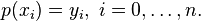
Given a set of n+1 data points (x_i,y_i) where no two x_i are the same, one is looking for a polynomial p of degree at most n with the property

$p(x_i) = y_i,\; i=0,\ldots,n.$

The unisolvence theorem states that such a polynomial p exists and is unique.

In more sophisticated terms, the theorem states that for n+1 interpolation nodes (x_i), polynomial interpolation defines a linear bijection

$L_n:\mathbb{K}^{n+1} \to \Pi_n$

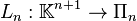
where $Π n$ is the vector space of polynomials with degree n or less.

[edit] Constructing the interpolation polynomial

The red dots denote the data points (x_k,y_k), while the blue curve shows the interpolation polynomial.

Suppose that the interpolation polynomial is in the form

$p(x) = a_n x^n + a_{n-1} x^{n-1} + \cdots + a_2 x^2 + a_1 x + a_0. \qquad (1)$

The statement that p interpolates the data points means that

$p(x_i) = y_i \qquad\mbox{for all } i \in \left\{ 0, 1, \dots, n\right\}.$

If we substitute equation (1) in here, we get a system of linear equations in the coefficients $a k$ . The system in matrix-vector form reads

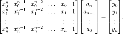
$\begin{bmatrix} x_0^n & x_0^{n-1} & x_0^{n-2} & \ldots & x_0 & 1 \\ x_1^n & x_1^{n-1} & x_1^{n-2} & \ldots & x_1 & 1 \\ \vdots & \vdots & \vdots & & \vdots & \vdots \\ x_n^n & x_n^{n-1} & x_n^{n-2} & \ldots & x_n & 1 \end{bmatrix} \begin{bmatrix} a_n \\ a_{n-1} \\ \vdots \\ a_0 \end{bmatrix} = \begin{bmatrix} y_0 \\ y_1 \\ \vdots \\ y_n \end{bmatrix}.$

We have to solve this system for $a k$ to construct the interpolant $p (x).$

The matrix on the left is commonly referred to as a Vandermonde matrix. Its determinant is nonzero, which proves the unisolvence theorem: there exists a unique interpolating polynomial.

The condition number of the Vandermonde matrix may be large,^[1] causing large errors when computing the coefficients $a i$ if the system of equations is solved using Gauss elimination. Several authors have therefore proposed algorithms which exploit the structure of the Vandermonde matrix to compute numerically stable solutions in $\mathcal O(n^2)$ operations instead of the $\mathcal O(n^3)$ required by Gaussian elimination.^[2]^[3]^[4] These methods rely on constructing first a Newton interpolation of the polynomial and then converting it to the monomial form above.

[edit] Non-Vandermonde solutions

We are trying to construct our unique interpolation polynomial in the vector space $Π n$ that is the vector space of polynomials of degree n. When using a monomial basis for $Π n$ we have to solve the Vandermonde matrix to construct the coefficients $a k$ for the interpolation polynomial. This can be a very costly operation (as counted in clock cycles of a computer trying to do the job). By choosing another basis for $Π n$ we can simplify the calculation of the coefficients but then we have to do additional calculations when we want to express the interpolation polynomial in terms of a monomial basis.

One method is to write the interpolation polynomial in the Newton form and use the method of divided differences to construct the coefficients, e.g. Neville's algorithm. The cost is O $(n 2)$ operations, while Gaussian elimination costs O $(n 3)$ operations. Furthermore, you only need to do O $(n)$ extra work if an extra point is added to the data set, while for the other methods, you have to redo the whole computation.

Another method is to use the Lagrange form of the interpolation polynomial. The resulting formula immediately shows that the interpolation polynomial exists under the conditions stated in the above theorem.

The Bernstein form was used in a constructive proof of the Weierstrass approximation theorem by Bernstein and has nowadays gained great importance in computer graphics in the form of Bezier curves.

[edit] Interpolation error

When interpolating a given function f by a polynomial of degree n at the nodes x₀,...,x_n we get the error

$f(x) - p_n(x) = f[x_0,\ldots,x_n,x] \prod_{i=0}^n (x-x_i)$

where

$f[x_0,\ldots,x_n,x]$

is the notation for divided differences. When f is n+1 times continuously differentiable on the smallest interval I which contains the nodes x_i and x then we can write the error in the Lagrange form as

$f(x) - p_n(x) = \frac{f^{(n+1)}(\xi)}{(n+1)!} \prod_{i=0}^n (x-x_i)$

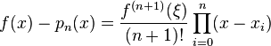
for some $ξ$ in I. Thus the remainder term in the Lagrange form of the Taylor theorem is a special case of interpolation error when all interpolation nodes x_i are identical.

In the case of equally spaced interpolation nodes $x i = x 0 + i h$ , it follows that the interpolation error is O $(h n)$ . However, this does not yield any information on what happens when $n \to \infty$ . That question is treated in the section Convergence properties.

The above error bound suggests choosing the interpolation points x_i such that the product | ∏ (x − x_i) | is as small as possible. The Chebyshev nodes achieve this.

[edit] Lebesgue constants

See the main article: Lebesgue constant.

We fix the interpolation nodes x₀, ..., x_n and an interval [a, b] containing all the interpolation nodes. The process of interpolation maps the function f to a polynomial p. This defines a mapping X from the space C([a, b]) of all continuous functions on [a, b] to itself. The map X is linear and it is a projection on the subspace Π_n of polynomials of degree n or less.

The Lebesgue constant L is defined as the operator norm of X. One has (a special case of Lebesgue's lemma):

$\|f-X(f)\| \le (L+1) \|f-p^*\|.$

In other words, the interpolation polynomial is at most a factor (L+1) worse than the best possible approximation. This suggests that we look for a set of interpolation nodes that L small. In particular, we have for Chebyshev nodes:

$L \ge \frac2\pi \log(n+1) + C \quad\mbox{for some constant } C.$

We conclude again that Chebyshev nodes are a very good choice for polynomial interpolation, as the growth in n is exponential for equidistant nodes. However, those nodes are not optimal.

[edit] Convergence properties

It is natural to ask, for which classes of functions and for which interpolation nodes the sequence of interpolating polynomials converges to the interpolated function as the degree n goes to infinity? Convergence may be understood in different ways, e.g. pointwise, uniform or in some integral norm.

The situation is rather bad for equidistant nodes, in that uniform convergence is not even guaranteed for infinitely differentiable functions. One classical example, due to Carle Runge, is the function f(x) = 1 / (1 + x²) considered on the interval [−5, 5]. The interpolation error ||f − p_n||_∞ grows without bound as n → ∞. Another example is the function f(x) = |x| on the interval [−1, 1], for which the interpolating polynomials do not even converge pointwise except at the three points x = −1, 0, and 1.^[5]

One might think that better convergence properties may be obtained by choosing different interpolation nodes. The following theorem seems to be a rather encouraging answer:

For any function f(x) continuous on an interval [a,b] there exists a table of nodes for which the sequence of interpolating polynomials

p n (x)

converges to f(x) uniformly on [a,b].

Proof. It's clear that the sequence of polynomials of best approximation $p^*_n(x)$ converges to f(x) uniformly (due to Weierstrass approximation theorem). Now we have only to show that each $p^*_n(x)$ may be obtained by means of interpolation on certain nodes. But this is true due to a special property of polynomials of best approximation known from the Chebyshev alternation theorem. Specifically, we know that such polynomials should intersect f(x) at least n+1 times. Choosing the points of intersection as interpolation nodes we obtain the interpolating polynomial coinciding with the best approximation polynomial.

The defect of this method, however, is that interpolation nodes should be calculated anew for each new function f(x), but the algorithm is hard to be implemented numerically. Does there exist a single table of nodes for which the sequence of interpolating polynomials converge to any continuous function f(x)? The answer is unfortunately negative as it is stated by the following theorem:

For any table of nodes there is a continuous function f(x) on an interval [a,b] for which the sequence of interpolating polynomials diverges on [a,b].^[6]

The proof essentially uses the lower bound estimation of the Lebesgue constant, which we defined above to be the operator norm of X_n (where X_n is the projection operator on Π_n). Now we seek a table of nodes for which

$\lim_{n \to \infty} X_n f = f,$ for any $f \in C([a,b]).$

Due to the Banach-Steinhaus theorem, this is only possible when norms of X_n are uniformly bounded, which cannot be true since we know that 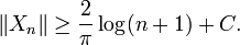$\|X_n\|\geq \frac{2}{\pi} \log(n+1)+C.$

For example, if equidistant points are chosen as interpolation nodes, the function from Runge's phenomenon demonstrates divergence of such interpolation. Note that this function is not only continuous but even infinitely times differentiable on [−1, 1]. For better Chebyshev nodes, however, such an example is much harder to find because of the theorem:

For every absolutely continuous function on [−1, 1] the sequence of interpolating polynomials constructed on Chebyshev nodes converges to f(x) uniformly.

[edit] Related concepts

Runge's phenomenon shows that for high values of n, the interpolation polynomial may oscillate wildly between the data points. This problem is commonly resolved by the use of spline interpolation. Here, the interpolant is not a polynomial but a spline: a chain of several polynomials of a lower degree.

Using harmonic functions to interpolate a periodic function is usually done using Fourier series, for example in discrete Fourier transform. This can be seen as a form of polynomial interpolation with harmonic base functions, see trigonometric interpolation and trigonometric polynomial.

Hermite interpolation problems are those where not only the values of the polynomial p at the nodes are given, but also all derivatives up to a given order, that is, it is prescribed there a whole k-jet. This turns out to be equivalent to a system of simultaneous polynomial congruences, and may be solved by means of the Chinese remainder theorem for polynomials. Birkhoff interpolation is a further generalization where only derivatives of some orders are prescribed, not necessarily all orders from 0 to a k.

Collocation methods for the solution of differential and integral equations are based on polynomial interpolation.

The technique of rational function modeling is a generalization that considers ratios of polynomial functions.

[edit] Notes

^ Gautschi, Walter (1975). "Norm Estimates for Inverses of Vandermonde Matrices". Numerische Mathematik 23: 337–347. doi:10.1007/BF01438260.
^ Higham, N. J. (1988). "Fast Solution of Vandermonde-Like Systems Involving Orthogonal Polynomials". IMA Journal of Numerical Analysis 8: 473–486. doi:10.1093/imanum/8.4.473.
^ Björck, Å; V. Pereyra (1970). "Solution of Vandermonde Systems of Equations". Mathematics of Computation 24 (112): 893–903. doi:10.2307/2004623.
^ Calvetti, D and Reichel, L (1993). "Fast Inversion of Vanderomnde-Like Matrices Involving Orthogonal Polynomials". BIT 33 (33): 473–484. doi:10.1007/BF01990529.
^ Watson (1980, p. 21) attributes the last example to Bernstein (1912).
^ Watson (1980, p. 21) attributes this theorem to Faber (1914).

[edit] References

Kendell A. Atkinson (1988). An Introduction to Numerical Analysis (2nd ed.), Chapter 3. John Wiley and Sons. ISBN 0-471-50023-2.
Sergei N. Bernstein (1912), Sur l'ordre de la meilleure approximation des fonctions continues par les polynômes de degré donné. Mem. Acad. Roy. Belg. 4, 1–104.
L. Brutman (1997), Lebesgue functions for polynomial interpolation — a survey, Ann. Numer. Math. 4, 111–127.
Georg Faber (1912), Über die interpolatorische Darstellung stetiger Funktionen, Deutsche Math. Jahr. 23, 192–210.
M.J.D. Powell (1981). Approximation Theory and Methods, Chapter 4. Cambridge University Press. ISBN 0-521-29514-9.
Michelle Schatzman (2002). Numerical Analysis: A Mathematical Introduction, Chapter 4. Clarendon Press, Oxford. ISBN 0-19-850279-6.
Endre Süli and David Mayers (2003). An Introduction to Numerical Analysis, Chapter 6. Cambridge University Press. ISBN 0-521-00794-1.
G. Alistair Watson (1980). Approximation Theory and Numerical Methods. John Wiley. ISBN 0-471-27706-1.

[edit] External links

Interpolating Polynomial by Stephen Wolfram, the Wolfram Demonstrations Project.

[0] Gautschi, Walter (1975). "Norm Estimates for Inverses of Vandermonde Matrices". Numerische Mathematik 23: 337–347. doi:10.1007/BF01438260.

[1] Higham, N. J. (1988). "Fast Solution of Vandermonde-Like Systems Involving Orthogonal Polynomials". IMA Journal of Numerical Analysis 8: 473–486. doi:10.1093/imanum/8.4.473.

[2] Björck, Å; V. Pereyra (1970). "Solution of Vandermonde Systems of Equations". Mathematics of Computation 24 (112): 893–903. doi:10.2307/2004623.

[3] Calvetti, D and Reichel, L (1993). "Fast Inversion of Vanderomnde-Like Matrices Involving Orthogonal Polynomials". BIT 33 (33): 473–484. doi:10.1007/BF01990529.

[4] Watson (1980, p. 21) attributes the last example to Bernstein (1912).

[5] Watson (1980, p. 21) attributes this theorem to Faber (1914).

[1]

[2]

[3]

[4]

[5]

[6]

Polynomial interpolation

From Wikipedia, the free encyclopedia

Contents

[edit] Applications

[edit] Definition

[edit] Constructing the interpolation polynomial

[edit] Non-Vandermonde solutions

[edit] Interpolation error

[edit] Lebesgue constants

[edit] Convergence properties

[edit] Related concepts

[edit] Notes

[edit] References

[edit] External links

Views

Personal tools

Navigation

Search

Interaction

Toolbox

Languages