%5Bwikipedia_article%5D 3d axis calibration coordinate developing eigen geometry graphics homogeneous images java linear linearalgebra math mathematics maths matrix misc:maths opengl polar.decomposition programming research rotation text transformation transformations usct visualisation

My tags:

From Wikipedia, the free encyclopedia

In linear algebra, a rotation matrix is any matrix that acts as a rotation of Euclidean space. For example, the matrix

rotates vectors in the plane counterclockwise by an angle of θ. In three dimensions, rotation matrices are among the simplest algebraic descriptions of rotations, and are used extensively for computations in geometry, physics, and computer graphics.

Though most applications involve rotations in 2 or 3 dimensions, rotation matrices can be defined for n-dimensional space. Algebraically, a rotation matrix is an orthogonal matrix whose determinant is equal to 1:

Rotation matrices are always square, and are usually assumed to have real entries, though the definition makes sense for other scalar fields. The set of all n × n rotation matrices forms a group, known as the rotation group (or special orthogonal group).

Contents 1 Rotations in two and three dimensions 1.1 Dimension two 1.2 Dimension three 1.3 Axis of a rotation 2 Properties of a rotation matrix 3 Examples 4 Geometry 5 Multiplication 6 Ambiguities 7 Decompositions 7.1 Independent planes 7.2 Sequential angles 7.3 Nested dimensions 7.4 Skew parameters 8 Lie theory 8.1 Lie group 8.2 Lie algebra 8.3 Exponential map 8.4 Baker–Campbell–Hausdorff formula 8.5 Spin group 9 Infinitesimal rotations 10 Conversions 10.1 Quaternion 10.2 Polar decomposition 10.3 Axis and angle 10.4 Euler angles 11 Uniform random rotation matrices 12 References 13 See also 14 External links

[edit] Rotations in two and three dimensions

[edit] Dimension two

In two dimensions, every rotation matrix has the following form:

This matrix rotates the plane counterclockwise around the origin by an angle of θ (assuming the standard right-handed coordinate system). For a clockwise rotation, simply replace θ by –θ:

Particularly useful are the matrices for 90° and 180° rotations:

[edit] Dimension three

There are three basic rotation matrices in three dimensions:

These matrices represent counterclockwise rotations of an object relative to fixed coordinate axes, by an angle of θ, around the x, y, and z axes, respectively. The direction of the rotation is determined by the right-hand rule: R_x rotates the y-axis towards the z-axis, R_y rotates the z-axis towards the x-axis, and R_z rotates the x-axis towards the y-axis. The transpose of the above matrices represents positive (right-hand sense) rotation of the coordinate axes relative to a fixed object.

Other rotation matrices can be obtained from these three using matrix multiplication. For example, the product

represents a rotation whose yaw, pitch, and roll are α, β, and γ, respectively. Similarly, the product

represents a rotation whose Euler angles are α, β, and γ (using the z-x-z convention for Euler angles). In both cases the matrices are assumed to act on column vectors.

[edit] Axis of a rotation

Every rotation in three dimensions has an axis — a direction that is fixed by the rotation. Given a rotation matrix R, a vector u in the direction of the axis can be found by solving the equation

For some applications, it is helpful to be able to make a rotation with a given axis. Given a unit vector u = (u_x, u_y, u_z), where u_x² + u_y² + u_z² = 1, the matrix for a counterclockwise rotation by an angle of θ about an axis the direction of u is^[1]:

where

This formula can be written as

where

and I is the 3 × 3 identity matrix. The matrix P is the projection onto the axis of rotation, and I – P is the projection onto the plane orthogonal to the axis.

[edit] Properties of a rotation matrix

The above discussion can be generalised to any number of dimensions. For any rotation matrix and I, the identity in

[edit] Examples

The 2×2 rotation matrix corresponds to a 90° planar rotation. The transpose of the 2×2 matrix is its inverse, but since its determinant is −1 this is not a rotation matrix; it is a reflection across the line 11y = 2x. The 3×3 rotation matrix corresponds to a −30° rotation around the x axis in three-dimensional space. The 3×3 rotation matrix corresponds to a rotation of approximately 74° around the axis (−1⁄3,2⁄3,2⁄3) in three-dimensional space. The 3×3 permutation matrix is also a rotation matrix, as is the matrix of any even permutation (but never of any odd permutation).

The 3×3 matrix has determinant +1, but its transpose is not its inverse, so it is not a rotation matrix. The 4×3 matrix is not square, and so cannot be a rotation matrix; yet QTQ yields a 3×3 identity matrix (the columns are orthonormal). The 4×4 rotation matrix has no axis of rotation; it reverses the direction of every vector. The 5×5 rotation matrix rotates vectors in the plane of the first two coordinate axes 90°, rotates vectors in the plane of the next two axes 180°, and leaves the last coordinate axis unmoved.

[edit] Geometry

In Euclidean geometry, a rotation is an example of an isometry, a transformation that moves points without changing the distances between them. Rotations are distinguished from other isometries by two additional properties: they leave (at least) one point fixed, and they leave "handedness" unchanged. By contrast, a translation moves every point, a reflection exchanges left- and right-handed ordering, and a glide reflection does both.

A rotation that does not leave "handedness" unchanged is called an Improper Rotation or a Rotoinversion

If we take the fixed point as the origin of a Cartesian coordinate system, then every point can be given coordinates as a displacement from the origin. Thus we may work with the vector space of displacements instead of the points themselves. Now suppose (p₁,…,p_n) are the coordinates of the vector p from the origin, O, to point P. Choose an orthonormal basis for our coordinates; then the squared distance to P, by Pythagoras, is

which we can compute using the matrix multiplication

A geometric rotation transforms lines to lines, and preserves ratios of distances between points. From these properties we can show that a rotation is a linear transformation of the vectors, and thus can be written in matrix form, Qp. The fact that a rotation preserves, not just ratios, but distances themselves, we can state as

or

Because this equation holds for all vectors, p, we conclude that every rotation matrix, Q, satisfies the orthogonality condition,

Rotations preserve handedness because they cannot change the ordering of the axes, which implies the special matrix condition,

Equally important, we can show that any matrix satisfying these two conditions acts as a rotation.

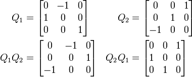
[edit] Multiplication

The inverse of a rotation matrix is its transpose, which is also a rotation matrix:

The product of two rotation matrices is a rotation matrix:

For n greater than 2, multiplication of n×n rotation matrices is not commutative.

Noting that any identity matrix is a rotation matrix, and that matrix multiplication is associative, we may summarize all these properties by saying that the n×n rotation matrices form a group, which for n > 2 is non-abelian. Called a special orthogonal group, and denoted by SO(n), SO(n,R), SO_n, or SO_n(R), the group of n×n rotation matrices is isomorphic to the group of rotations in an n-dimensional space. This means that multiplication of rotation matrices corresponds to composition of rotations, applied in left-to-right order of their corresponding matrices.

[edit] Ambiguities

The interpretation of a rotation matrix can be subject to many ambiguities.

Alias or alibi transformation

The change in a vector's coordinates can indicate a turn of the coordinate system (alias) or a turn of the vector (alibi).

Right- or left-handed coordinates

The matrix can be with respect to a right-handed or left-handed coordinate system.

World or body axes

The coordinate axes can be fixed or rotate with a body.

Vectors or forms

The vector space has a dual space of linear forms, and the matrix can act on either vectors or forms.

In most cases the effect of the ambiguity is to transpose or invert the matrix.

[edit] Decompositions

[edit] Independent planes

Consider the 3×3 rotation matrix

If Q acts in a certain direction, v, purely as a scaling by a factor λ, then we have

so that

Thus λ is a root of the characteristic polynomial for Q,

Two features are noteworthy. First, one of the roots (or eigenvalues) is 1, which tells us that some direction is unaffected by the matrix. For rotations in three dimensions, this is the axis of the rotation (a concept that has no meaning in any other dimension). Second, the other two roots are a pair of complex conjugates, whose product is 1 (the constant term of the quadratic), and whose sum is 2 cos θ (the negated linear term). This factorization is of interest for 3×3 rotation matrices because the same thing occurs for all of them. (As special cases, for a null rotation the "complex conjugates" are both 1, and for a 180° rotation they are both −1.) Furthermore, a similar factorization holds for any n×n rotation matrix. If the dimension, n, is odd, there will be a "dangling" eigenvalue of 1; and for any dimension the rest of the polynomial factors into quadratic terms like the one here (with the two special cases noted). We are guaranteed that the characteristic polynomial will have degree n and thus n eigenvalues. And since a rotation matrix commutes with its transpose, it is a normal matrix, so can be diagonalized. We conclude that every rotation matrix, when expressed in a suitable coordinate system, partitions into independent rotations of two-dimensional subspaces, at most ⁿ⁄₂ of them.

The sum of the entries on the main diagonal of a matrix is called the trace; it does not change if we reorient the coordinate system, and always equals the sum of the eigenvalues. This has the convenient implication for 2×2 and 3×3 rotation matrices that the trace reveals the angle of rotation, θ, in the two-dimensional (sub-)space. For a 2×2 matrix the trace is 2 cos(θ), and for a 3×3 matrix it is 1+2 cos(θ). In the three-dimensional case, the subspace consists of all vectors perpendicular to the rotation axis (the invariant direction, with eigenvalue 1). Thus we can extract from any 3×3 rotation matrix a rotation axis and an angle, and these completely determine the rotation.

[edit] Sequential angles

The constraints on a 2×2 rotation matrix imply that it must have the form

with a²+b² = 1. Therefore we may set a = cos θ and b = sin θ, for some angle θ. To solve for θ it is not enough to look at a alone or b alone; we must consider both together to place the angle in the correct quadrant, using a two-argument arctangent function.

Now consider the first column of a 3×3 rotation matrix,

Although a²+b² will probably not equal 1, but some value r² < 1, we can use a slight variation of the previous computation to find a so-called Givens rotation that transforms the column to

zeroing b. This acts on the subspace spanned by the x and y axes. We can then repeat the process for the xz subspace to zero c. Acting on the full matrix, these two rotations produce the schematic form

Shifting attention to the second column, a Givens rotation of the yz subspace can now zero the z value. This brings the full matrix to the form

which is an identity matrix. Thus we have decomposed Q as

An n×n rotation matrix will have (n−1)+(n−2)+⋯+2+1, or

entries below the diagonal to zero. We can zero them by extending the same idea of stepping through the columns with a series of rotations in a fixed sequence of planes. We conclude that the set of n×n rotation matrices, each of which has n² entries, can be parameterized by n(n−1)/2 angles.

xzxw	xzyw	xyxw	xyzw
yxyw	yxzw	yzyw	yzxw
zyzw	zyxw	zxzw	zxyw
xzxb	yzxb	xyxb	zyxb
yxyb	zxyb	yzyb	xzyb
zyzb	xyzb	zxzb	yxzb

In three dimensions this restates in matrix form an observation made by Euler, so mathematicians call the ordered sequence of three angles Euler angles. However, the situation is somewhat more complicated than we have so far indicated. Despite the small dimension, we actually have considerable freedom in the sequence of axis pairs we use; and we also have some freedom in the choice of angles. Thus we find many different conventions employed when three-dimensional rotations are parameterized for physics, or medicine, or chemistry, or other disciplines. When we include the option of world axes or body axes, 24 different sequences are possible. And while some disciplines call any sequence Euler angles, others give different names (Euler, Cardano, Tait-Byan, roll-pitch-yaw) to different sequences.

One reason for the large number of options is that, as noted previously, rotations in three dimensions (and higher) do not commute. If we reverse a given sequence of rotations, we get a different outcome. This also implies that we cannot compose two rotations by adding their corresponding angles. Thus Euler angles are not vectors, despite a similarity in appearance as a triple of numbers.

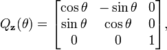
[edit] Nested dimensions

A 3×3 rotation matrix like

suggests a 2×2 rotation matrix,

is embedded in the upper left corner:

This is no illusion; not just one, but many, copies of n-dimensional rotations are found within (n+1)-dimensional rotations, as subgroups. Each embedding leaves one direction fixed, which in the case of 3×3 matrices is the rotation axis. For example, we have

fixing the x axis, the y axis, and the z axis, respectively. The rotation axis need not be a coordinate axis; if u = (x,y,z) is a unit vector in the desired direction, then

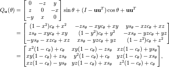
where c_θ = cos θ, s_θ = sin θ, is a rotation by angle θ leaving axis u fixed.

A direction in (n+1)-dimensional space will be a unit magnitude vector, which we may consider a point on a generalized sphere, Sⁿ. Thus it is natural to describe the rotation group SO(n+1) as combining SO(n) and Sⁿ. A suitable formalism is the fiber bundle,

where for every direction in the "base space", Sⁿ, the "fiber" over it in the "total space", SO(n+1), is a copy of the "fiber space", SO(n), namely the rotations that keep that direction fixed.

Thus we can build an n×n rotation matrix by starting with a 2×2 matrix, aiming its fixed axis on S² (the ordinary sphere in three-dimensional space), aiming the resulting rotation on S³, and so on up through Sⁿ⁻¹. A point on Sⁿ can be selected using n numbers, so we again have n(n−1)/2 numbers to describe any n×n rotation matrix.

In fact, we can view the sequential angle decomposition, discussed previously, as reversing this process. The composition of n−1 Givens rotations brings the first column (and row) to (1,0,…,0), so that the remainder of the matrix is a rotation matrix of dimension one less, embedded so as to leave (1,0,…,0) fixed.

[edit] Skew parameters

When an n×n rotation matrix, Q, does not include −1 as an eigenvalue, so that none of the planar rotations of which it is composed are 180° rotations, then Q+I is an invertible matrix. Most rotation matrices fit this description, and for them we can show that (Q−I)(Q+I)⁻¹ is a skew-symmetric matrix, A. Thus A^T = −A; and since the diagonal is necessarily zero, and since the upper triangle determines the lower one, A contains n(n−1)/2 independent numbers. Conveniently, I−A is invertible whenever A is skew-symmetric; thus we can recover the original matrix using the Cayley transform,

which maps any skew-symmetric matrix A to a rotation matrix. In fact, aside from the noted exceptions, we can produce any rotation matrix in this way. Although in practical applications we can hardly afford to ignore 180° rotations, the Cayley transform is still a potentially useful tool, giving a parameterization of most rotation matrices without trigonometric functions.

In three dimensions, for example, we have (Cayley 1846)

If we condense the skew entries into a vector, (x,y,z), then we produce a 90° rotation around the x axis for (1,0,0), around the y axis for (0,1,0), and around the z axis for (0,0,1). The 180° rotations are just out of reach; for, in the limit as x goes to infinity, (x,0,0) does approach a 180° rotation around the x axis, and similarly for other directions.

[edit] Lie theory

[edit] Lie group

We have established that n×n rotation matrices form a group, the special orthogonal group, SO(n). This algebraic structure is coupled with a topological structure, in that the operations of multiplication and taking the inverse (which here is merely transposition) are continuous functions of the matrix entries. Thus SO(n) is a classic example of a topological group. (In purely topological terms, it is a compact manifold.) Furthermore, the operations are not only continuous, but smooth, so SO(n) is a differentiable manifold and a Lie group (Baker (2003); Fulton & Harris (1991)).

Most properties of rotation matrices depend very little on the dimension, n; yet in Lie group theory we see systematic differences between even dimensions and odd dimensions. As well, there are some irregularities below n = 5; for example, SO(4) is, anomalously, not a simple Lie group, but instead isomorphic to the product of S³ and SO(3).

[edit] Lie algebra

Associated with every Lie group is a Lie algebra, a linear space equipped with a bilinear alternating product called a bracket. The algebra for SO(n) is denoted by

and consists of all skew-symmetric n×n matrices (as implied by differentiating the orthogonality condition, I = Q^TQ). The bracket, [A₁,A₂], of two skew-symmetric matrices is defined to be A₁A₂−A₂A₁, which is again a skew-symmetric matrix. This Lie algebra bracket captures the essence of the Lie group product via infinitesimals.

For 2×2 rotation matrices, the Lie algebra is a one-dimensional vector space, multiples of

Here the bracket always vanishes, which tells us that, in two dimensions, rotations commute. Not so in any higher dimension. For 3×3 rotation matrices, we have a three-dimensional vector space with the convenient basis (generators)

The essence of the bracket for these basis vectors works out to be as follows.

We can conveniently identify any matrix in this Lie algebra with a vector in R³,

Under this identification, the so(3) bracket has a memorable description; it is the vector cross product,

The matrix identified with a vector v is also memorable, because

Notice this implies that v is in the null space of the skew-symmetric matrix with which it is identified, because v×v is always the zero vector.

[edit] Exponential map

Connecting the Lie algebra to the Lie group is the exponential map, which we define using the familiar power series for e^x (Wedderburn 1934, §8.02),

For any skew-symmetric A, exp(A) is always a rotation matrix.

An important practical example is the 3×3 case, where we have seen we can identify every skew-symmetric matrix with a vector ω = uθ, where u = (x,y,z) is a unit magnitude vector. Recall that u is in the null space of the matrix associated with ω, so that if we use a basis with u as the z axis the final column and row will be zero. Thus we know in advance that the exponential matrix must leave u fixed. It is mathematically impossible to supply a straightforward formula for such a basis as a function of u (its existence would violate the hairy ball theorem), but direct exponentiation is possible, and yields

where c = cos ^θ⁄₂, s = sin ^θ⁄₂. We recognize this as our matrix for a rotation around axis u by angle θ. We also note that this mapping of skew-symmetric matrices is quite different from the Cayley transform discussed earlier.

In any dimension, if we choose some nonzero A and consider all its scalar multiples, exponentiation yields rotation matrices along a geodesic of the group manifold, forming a one-parameter subgroup of the Lie group. More broadly, the exponential map provides a homeomorphism between a neighborhood of the origin in the Lie algebra and a neighborhood of the identity in the Lie group. In fact, we can produce any rotation matrix as the exponential of some skew-symmetric matrix, so for these groups the exponential map is a surjection.

[edit] Baker–Campbell–Hausdorff formula

Suppose we are given A and B in the Lie algebra. Their exponentials, exp(A) and exp(B), are rotation matrices, which we can multiply. Since the exponential map is a surjection, we know that for some C in the Lie algebra, exp(A)exp(B) = exp(C), and we write

When exp(A) and exp(B) commute (which always happens for 2×2 matrices, but not higher), then C = A+B, mimicking the behavior of complex exponentiation. The general case is given by the BCH formula, a series expanded in terms of the bracket (Hall 2004, Ch. 3; Varadarajan 1984, §2.15). For matrices, the bracket is the same operation as the commutator, which detects lack of commutativity in multiplication. The general formula begins as follows.

Representation of a rotation matrix as a sequential angle decomposition, as in Euler angles, may tempt us to treat rotations as a vector space, but the higher order terms in the BCH formula reveal that to be a mistake.

We again take special interest in the 3×3 case, where [A,B] equals the cross product, A×B. If A and B are linearly independent, then A, B, and A×B can be used as a basis; if not, then A and B commute. And conveniently, in this dimension the summation in the BCH formula has a closed form (Engø 2001) as αA+βB+γ(A×B).

[edit] Spin group

The Lie group of n×n rotation matrices, SO(n), is a compact and path-connected manifold, and thus locally compact and connected. However, it is not simply connected, so Lie theory tells us it is a kind of "shadow" (a homomorphic image) of a universal covering group. Often the covering group, which in this case is the spin group denoted by Spin(n), is simpler and more natural to work with (Baker 2003, Ch. 5; Fulton & Harris 1991, pp. 299–315).

In the case of planar rotations, SO(2) is topologically a circle, S¹. Its universal covering group, Spin(2), is isomorphic to the real line, R, under addition. In other words, whenever we use angles of arbitrary magnitude, which we often do, we are essentially taking advantage of the convenience of the "mother space". Every 2×2 rotation matrix is produced by a countable infinity of angles, separated by integer multiples of 2π. Correspondingly, the fundamental group of SO(2) is isomorphic to the integers, Z.

In the case of spatial rotations, SO(3) is topologically equivalent to three-dimensional real projective space, RP³. Its universal covering group, Spin(3), is isomorphic to the 3-sphere, S³. Every 3×3 rotation matrix is produced by two opposite points on the sphere. Correspondingly, the fundamental group of SO(2) is isomorphic to the two-element group, Z₂. We can also describe Spin(3) as isomorphic to quaternions of unit norm under multiplication, or to certain 4×4 real matrices, or to 2×2 complex special unitary matrices.

Concretely, a unit quaternion, q, with

produces the rotation matrix

This is our third version of this matrix, here as a rotation around non-unit axis vector (x,y,z) by angle 2θ, where cos θ = w and |sin θ| = ||(x,y,z)||. (The proper sign for sin θ is implied once the signs of the axis components are decided.)

Many features of this case are the same for higher dimensions. The coverings are all two-to-one, with SO(n), n > 2, having fundamental group Z₂. The natural setting for these groups is within a Clifford algebra. And the action of the rotations is produced by a kind of "sandwich", denoted by qvq^∗.

[edit] Infinitesimal rotations

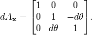
The matrices in the Lie algebra are not themselves rotations; the skew-symmetric matrices are derivatives, proportional differences of rotations. An actual "differential rotation", or infinitesimal rotation matrix has the form

where dθ is vanishingly small. These matrices do not satisfy all the same properties as ordinary finite rotation matrices under the usual treatment of infinitesimals (Goldstein, Poole & Safko 2002, §4.8). To understand what this means, consider

We first test the orthogonality condition, Q^TQ = I. The product is

differing from an identity matrix by second order infinitesimals, which we discard. So to first order, an infinitesimal rotation matrix is an orthogonal matrix. Next we examine the square of the matrix.

Again discarding second order effects, we see that the angle simply doubles. This hints at the most essential difference in behavior, which we can exhibit with the assistance of a second infinitesimal rotation,

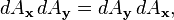
Compare the products dA_xdA_y and dA_ydA_x.

Since dθ dφ is second order, we discard it; thus, to first order, multiplication of infinitesimal rotation matrices is commutative. In fact,

again to first order.

But we must always be careful to distinguish (the first order treatment of) these infinitesimal rotation matrices from both finite rotation matrices and from derivatives of rotation matrices (namely skew-symmetric matrices). Contrast the behavior of finite rotation matrices in the BCH formula with that of infinitesimal rotation matrices, where all the commutator terms will be second order infinitesimals so we do have a vector space.

[edit] Conversions

We have seen the existence of several decompositions that apply in any dimension, namely independent planes, sequential angles, and nested dimensions. In all these cases we can either decompose a matrix or construct one. We have also given special attention to 3×3 rotation matrices, and these warrant further attention, in both directions (Stuelpnagel 1964).

[edit] Quaternion

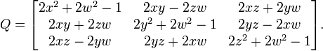
Rewrite the 3×3 rotation matrix again, as

Now every quaternion component appears multiplied by two in a term of degree two, and if all such terms are zero what's left is an identity matrix. This leads to an efficient, robust conversion from any quaternion — whether unit, nonunit, or even zero — to a 3×3 rotation matrix.

Nq = w^2 + x^2 + y^2 + z^2
if Nq > 0.0 then s = 2/Nq else s = 0.0
X = x*s; Y = y*s; Z = z*s
wX = w*X; wY = w*Y; wZ = w*Z
xX = x*X; xY = x*Y; xZ = x*Z
yY = y*Y; yZ = y*Z; zZ = z*Z
[ 1.0-(yY+zZ)   xY-wZ      xZ+wY    ]
[    xY+wZ   1.0-(xX+zZ)   yZ-wX    ]
[    xZ-wY      yZ+wX   1.0-(xX+yY) ]

Freed from the demand for a unit quaternion, we find that nonzero quaternions act as homogeneous coordinates for 3×3 rotation matrices. The Cayley transform, discussed earlier, is obtained by scaling the quaternion so that its w component is 1. For a 180° rotation around any axis, w will be zero, which explains the Cayley limitation.

The sum of the entries along the main diagonal (the trace), plus one, equals 4−4(x²+y²+z²), which is 4w². Thus we can write the trace itself as 2w²+2w²−1; and from the previous version of the matrix we see that the diagonal entries themselves have the same form: 2x²+2w²−1, 2y²+2w²−1, and 2z²+2w²−1. So we can easily compare the magnitudes of all four quaternion components using the matrix diagonal. We can, in fact, obtain all four magnitudes using sums and square roots, and choose consistent signs using the skew-symmetric part of the off-diagonal entries.

w = 0.5*sqrt(1+Qxx+Qyy+Qzz)
x = copysign(0.5*sqrt(1+Qxx-Qyy-Qzz),Qzy-Qyz)
y = copysign(0.5*sqrt(1-Qxx+Qyy-Qzz),Qxz-Qzx)
z = copysign(0.5*sqrt(1-Qxx-Qyy+Qzz),Qyx-Qxy)

where copysign(x,y) is x with the sign of y:

copysign(x,y)

Alternatively, use a single square root and division

t = Qxx+Qyy+Qzz
r = sqrt(1+t)
s = 0.5/r
w = 0.5*r
x = (Qzy-Qyz)*s
y = (Qxz-Qzx)*s
z = (Qyx-Qxy)*s

This is numerically stable so long as the trace, t, is not negative; otherwise, we risk dividing by (nearly) zero. In that case, suppose Q_xx is the largest diagonal entry, so x will have the largest magnitude (the other cases are similar); then the following is safe.

r = sqrt(1+Qxx-Qyy-Qzz)
s = 0.5/r
w = (Qzy-Qyz)*s
x = 0.5*r
y = (Qxy+Qyx)*s
z = (Qzx+Qxz)*s

If the matrix contains significant error, such as accumulated numerical error, we may construct a symmetric 4×4 matrix,

and find the eigenvector, (x,y,z,w), of its largest magnitude eigenvalue. (If Q is truly a rotation matrix, that value will be 1.) The quaternion so obtained will correspond to the rotation matrix closest to the given matrix (Bar-Itzhack 2000).

[edit] Polar decomposition

If the n×n matrix M is non-singular, its columns are linearly independent vectors; thus the Gram–Schmidt process can adjust them to be an orthonormal basis. Stated in terms of numerical linear algebra, we convert M to an orthogonal matrix, Q, using QR decomposition. However, we often prefer a Q "closest" to M, which this method does not accomplish. For that, the tool we want is the polar decomposition (Fan & Hoffman 1955; Higham 1989).

To measure closeness, we may use any matrix norm invariant under orthogonal transformations. A convenient choice is the Frobenius norm, ||Q−M||_F, squared, which is the sum of the squares of the element differences. Writing this in terms of the trace, Tr, our goal is,

• Find Q minimizing Tr( (Q−M)^T(Q−M) ), subject to Q^TQ = I.

Though written in matrix terms, the objective function is just a quadratic polynomial. We can minimize it in the usual way, by finding where its derivative is zero. For a 3×3 matrix, the orthogonality constraint implies six scalar equalities that the entries of Q must satisfy. To incorporate the constraint(s), we may employ a standard technique, Lagrange multipliers, assembled as a symmetric matrix, Y. Thus our method is:

• Differentiate Tr( (Q−M)^T(Q−M) + (Q^TQ−I)Y ) with respect to (the entries of) Q, and equate to zero.

In general, we obtain the equation

so that

where Q is orthogonal and S is symmetric. To ensure a minimum, the Y matrix (and hence S) must be positive definite. Linear algebra calls QS the polar decomposition of M, with S the positive square root of S² = M^TM.

When M is non-singular, the Q and S factors of the polar decomposition are uniquely determined. However, the determinant of S is positive because S is positive definite, so Q inherits the sign of the determinant of M. That is, Q is only guaranteed to be orthogonal, not a rotation matrix. This is unavoidable; an M with negative determinant has no uniquely-defined closest rotation matrix.

[edit] Axis and angle

To efficiently construct a rotation matrix from an angle θ and a unit axis u, we can take advantage of symmetry and skew-symmetry within the entries.

c = cos(θ); s = sin(θ); C = 1-c
xs = x*s;   ys = y*s;   zs = z*s
xC = x*C;   yC = y*C;   zC = z*C
xyC = x*yC; yzC = y*zC; zxC = z*xC
[ x*xC+c   xyC-zs   zxC+ys ]
[ xyC+zs   y*yC+c   yzC-xs ]
[ zxC-ys   yzC+xs   z*zC+c ]

Determining an axis and angle, like determining a quaternion, is only possible up to sign; that is, (u,θ) and (−u,−θ) correspond to the same rotation matrix, just like q and −q. As well, axis-angle extraction presents additional difficulties. The angle can be restricted to be from 0° to 180°, but angles are formally ambiguous by multiples of 360°. When the angle is zero, the axis is undefined. When the angle is 180°, the matrix becomes symmetric, which has implications in extracting the axis. Near multiples of 180°, care is needed to avoid numerical problems: in extracting the angle, a two-argument arctangent with atan2(sin θ,cos θ) equal to θ avoids the insensitivity of arccosine; and in computing the axis magnitude to force unit magnitude, a brute-force approach can lose accuracy through underflow (Moler & Morrison 1983).

A partial approach is as follows.

x = Qzy-Qyz
y = Qxz-Qzx
z = Qyx-Qxy
r = hypot(x,hypot(y,z))
t = Qxx+Qyy+Qzz
θ = atan2(r,t−1)

The x, y, and z components of the axis would then be divided by r. A fully robust approach will use different code when t is negative, as with quaternion extraction. When r is zero because the angle is zero, an axis must be provided from some source other than the matrix.

[edit] Euler angles

Complexity of conversion escalates with Euler angles (used here in the broad sense). The first difficulty is to establish which of the twenty-four variations of Cartesian axis order we will use. Suppose the three angles are θ₁, θ₂, θ₃; physics and chemistry may interpret these as

while aircraft dynamics may use

One systematic approach begins with choosing the right-most axis. Among all permutations of (x,y,z), only two place that axis first; one is an even permutation and the other odd. Choosing parity thus establishes the middle axis. That leaves two choices for the left-most axis, either duplicating the first or not. These three choices gives us 3×2×2 = 12 variations; we double that to 24 by choosing static or rotating axes.

This is enough to construct a matrix from angles, but triples differing in many ways can give the same rotation matrix. For example, suppose we use the zyz convention above; then we have the following equivalent pairs:

(90°,	45°,	−105°)	≡	(−270°,	−315°,	255°)	multiples of 360°
(72°,	0°,	0°)	≡	(40°,	0°,	32°)	singular alignment
(45°,	60°,	−30°)	≡	(−135°,	−60°,	150°)	bistable flip

The problem of singular alignment, the mathematical analog of physical gimbal lock, occurs when the middle rotation aligns the axes of the first and last rotations. It afflicts every axis order at either even or odd multiples of 90°, causing Euler angles to be abandoned for quaternions in many applications. Setting these unavoidable issues aside, angles for any order can be found using a concise common routine (Herter & Lott 1993; Shoemake 1994).

[edit] Uniform random rotation matrices

We sometimes need to generate a uniformly distributed random rotation matrix. It seems intuitively clear in two dimensions that this means the rotation angle is uniformly distributed between 0 and 2π. That intuition is correct, but does not carry over to higher dimensions. For example, if we decompose 3×3 rotation matrices in axis-angle form, the angle should not be uniformly distributed; the probability that (the magnitude of) the angle is at most θ should be ¹⁄_π(θ − sin θ), for 0 ≤ θ ≤ π.

Since SO(n) is a connected and locally compact Lie group, we have a simple standard criterion for uniformity, namely that the distribution be unchanged when composed with any arbitrary rotation (a Lie group "translation"). This definition corresponds to what is called Haar measure. León, Massé & Rivest (2006) show how to use the Cayley transform to generate and test matrices according to this criterion.

We can also generate a uniform distribution in any dimension using the subgroup algorithm of Diaconis & Shashahani (1987). This recursively exploits the nested dimensions group structure of SO(n), as follows. Generate a uniform angle and construct a 2×2 rotation matrix. To step from n to n+1, generate a vector v uniformly distributed on the n-sphere, Sⁿ, embed the n×n matrix in the next larger size with last column (0,…,0,1), and rotate the larger matrix so the last column becomes v.

As usual, we have special alternatives for the 3×3 case. Each of these methods begins with three independent random scalars uniformly distributed on the unit interval. Arvo (1992) takes advantage of the odd dimension to change a Householder reflection to a rotation by negation, and uses that to aim the axis of a uniform planar rotation.

Another method uses unit quaternions. Multiplication of rotation matrices is homomorphic to multiplication of quaternions, and multiplication by a unit quaternion rotates the unit sphere. Since the homomorphism is a local isometry, we immediately conclude that to produce a uniform distribution on SO(3) we may use a uniform distribution on S³.

Euler angles can also be used, though not with each angle uniformly distributed (Murnaghan 1962; Miles 1965).

For the axis-angle form, the axis is uniformly distributed over the unit sphere of directions, S², while the angle has the non-uniform distribution over [0,π] noted previously (Miles 1965).

[edit] References

• Arvo, James (1992), "Fast random rotation matrices", in David Kirk, Graphics Gems III, San Diego: Academic Press Professional, pp. 117–120, ISBN 978-0-12-409671-4, http://www.graphicsgems.org/ 
• Baker, Andrew (2003), Matrix Groups: An Introduction to Lie Group Theory, Springer, ISBN 978-1-85233-470-3 
• Bar-Itzhack, Itzhack Y. (Nov.–Dec. 2000), "New method for extracting the quaternion from a rotation matrix", AIAA Journal of Guidance, Control and Dynamics 23 (6): 1085–1087 (Engineering Note), ISSN 0731-5090 
• Björck, A.; Bowie, C. (June 1971), "An iterative algorithm for computing the best estimate of an orthogonal matrix", SIAM Journal on Numerical Analysis 8 (2): 358–364, ISSN 0036-1429 
• Cayley, Arthur (1846), "Sur quelques propriétés des déterminants gauches", Journal für die Reine und Angewandte Mathematik (Crelle's Journal), 32: 119–123, ISSN 0075-4102 ; reprinted as article 52 in Cayley, Arthur (1889), The collected mathematical papers of Arthur Cayley, I (1841–1853), Cambridge University Press, pp. 332–336, http://www.hti.umich.edu/cgi/t/text/pageviewer-idx?c=umhistmath;cc=umhistmath;rgn=full%20text;idno=ABS3153.0001.001;didno=ABS3153.0001.001;view=image;seq=00000349 
• Diaconis, Persi; Shahshahani, Mehrdad (1987), "The subgroup algorithm for generating uniform random variables", Probability in the Engineering and Informational Sciences 1: 15–32, ISSN 0269-9648 
• Engø, Kenth (June 2001), "On the BCH-formula in so(3)", BIT Numerical Mathematics 41 (3): 629–632, doi:10.1023/A:1021979515229, ISSN 0006-3835, http://www.ii.uib.no/publikasjoner/texrap/abstract/2000-201.html 
• Fan, Ky; Hoffman, Alan J. (February 1955), "Some metric inequalities in the space of matrices", Proc. AMS 6 (1): 111–116, doi:10.2307/2032662, ISSN 0002-9939 
• Fulton, William; Harris, Joe (1991), Representation Theory: A First Course, GTM, 129, New York, Berlin, Heidelberg: Springer, MR1153249, ISBN 978-0-387-97495-8 
• Goldstein, Herbert; Poole, Charles P.; Safko, John L. (2002), Classical Mechanics (third ed.), Addison Wesley, ISBN 978-0-201-65702-9 
• Hall, Brian C. (2004), Lie Groups, Lie Algebras, and Representations: An Elementary Introduction, Springer, ISBN 978-0-387-40122-5  (GTM 222)
• Herter, Thomas; Lott, Klaus (September–October 1993), "Algorithms for decomposing 3-D orthogonal matrices into primitive rotations", Computers & Graphics 17 (5): 517–527, ISSN 0097-8493 
• Higham, Nicholas J. (October 1 1989), "Matrix nearness problems and applications", in Gover, M. J. C.; Barnett, S., Applications of Matrix Theory, Oxford University Press, pp. 1–27, ISBN 978-0-19-853625-3, http://www.maths.manchester.ac.uk/~higham/pap-misc.html 
• León, Carlos A.; Massé, Jean-Claude; Rivest, Louis-Paul (February 2006), "A statistical model for random rotations", Journal of Multivariate Analysis 97 (2): 412–430, doi:10.1016/j.jmva.2005.03.009, ISSN 0047-259X, http://archimede.mat.ulaval.ca/pages/lpr/ 
• Miles, R. E. (December 1965), "On random rotations in R³", Biometrika 52 (3/4): 636–639, doi:10.2307/2333716, ISSN 0006-3444 
• Moler, Cleve; Morrison, Donald (1983), "Replacing square roots by pythagorean sums", IBM Journal of Research and Development 27 (6), ISSN 0018-8646, http://domino.watson.ibm.com/tchjr/journalindex.nsf/0b9bc46ed06cbac1852565e6006fe1a0/0043d03ee1c1013c85256bfa0067f5a6?OpenDocument 
• Murnaghan, Francis D. (1950), "The element of volume of the rotation group", Proceedings of the National Academy of Sciences 36 (11): 670–672, ISSN 0027-8424, http://www.pnas.org/content/vol36/issue11/ 
• Murnaghan, Francis D. (1962), The Unitary and Rotation Groups, Lectures on applied mathematics, Washington: Spartan Books 
• Prentice, Michael J. (1986), "Orientation statistics without parametric assumptions", Journal of the Royal Statistical Society. Series B (Methodological) 48 (2): 214–222, ISSN 0035-9246 
• Shepperd, Stanley W. (May–June 1978), "Quaternion from rotation matrix", AIAA Journal of Guidance, Control and Dynamics 1 (3): 223–224, ISSN 0731-5090 
• Shoemake, Ken (1994), "Euler angle conversion", in Paul Heckbert, Graphics Gems IV, San Diego: Academic Press Professional, pp. 222–229, ISBN 978-0-12-336155-4, http://www.graphicsgems.org/ 
• Stuelpnagel, John (October 1964), "On the parameterization of the three-dimensional rotation group", SIAM Review 6 (4): 422–430, ISSN 0036-1445  (Also NASA-CR-53568.)
• Varadarajan, V. S. (1984), Lie Groups, Lie Algebras, and Their Representation, Springer, ISBN 978-0-387-90969-1  (GTM 102)
• Wedderburn, J. H. M. (1934), Lectures on Matrices, AMS, ISBN 978-0-8218-3204-2, http://www.ams.org/online_bks/coll17/ 

[edit] See also

• Rotation
• Rotation representation
• Rotation group
• Isometry
• Orthogonal matrix
• Rodrigues' rotation formula
• Yaw-pitch-roll system

[edit] External links

• Rotation matrices at Mathworld
• Math Awareness Month 2000 interactive demo (requires Java)
• Rotation Matrices at MathPages