Invertible matrix

From Wikipedia, the free encyclopedia

In linear algebra, an n-by-n (square) matrix A is called invertible or non-singular if there exists an n-by-n matrix B such that

$\mathbf{AB} = \mathbf{BA} = \mathbf{I}_n \$

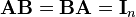
where I_n denotes the n-by-n identity matrix and the multiplication used is ordinary matrix multiplication. If this is the case, then the matrix B is uniquely determined by A and is called the inverse of A, denoted by A⁻¹. It follows from the theory of matrices that if

$\mathbf{AB} = \mathbf{I} \$

for square matrices A and B, then also

$\mathbf{BA} = \mathbf{I} \ .$ ^[1]

Non-square matrices (m-by-n matrices for which m ≠ n) do not have an inverse. However, in some cases such a matrix may have a left inverse or right inverse. If A is m-by-n and the rank of A is equal to n, then A has a left inverse: an n-by-m matrix B such that BA = I. If A has rank m, then it has a right inverse: an n-by-m matrix B such that AB = I.

While the most common case is that of matrices over the real or complex numbers, all these definitions can be given for matrices over any commutative ring.

A square matrix that is not invertible is called singular or degenerate. A square matrix is singular if and only if its determinant is 0. Singular matrices are rare in the sense that if you pick a random square matrix, it will almost surely not be singular (the precise meaning of this statement is given below).

Matrix inversion is the process of finding the matrix B that satisfies the prior equation for a given invertible matrix A.

[edit] Properties of invertible matrices

Let A be a square n by n matrix over a field $K$ (for example the field $R$ of real numbers). Then the following statements are equivalent:

A is invertible.

A is row-equivalent to the n-by-n identity matrix I_n.

A is column-equivalent to the n-by-n identity matrix I_n.

A has n pivot positions.

det A ≠ 0.

rank A = n.

The equation Ax = 0 has only the trivial solution x = 0 (i.e., Null A = {0})

The equation Ax = b has exactly one solution for each b in

K n

.

The columns of A are linearly independent.

The columns of A span

K n

(i.e. Col A =

K n

).

The columns of A form a basis of

K n

.

The linear transformation mapping x to Ax is a bijection from

K n

to

K n

.

There is an n by n matrix B such that AB = I_n.

The transpose A^T is an invertible matrix.

The matrix times its transpose, A^T × A is an invertible matrix.

The number 0 is not an eigenvalue of A.

In general, a square matrix over a commutative ring is invertible if and only if its determinant is a unit in that ring.

$\left(\mathbf{A}^{-1}\right)^{-1} = \mathbf{A}$ .
$\left(k\mathbf{A}\right)^{-1} = k^{-1}\mathbf{A}^{-1}$ .
$(\mathbf{A}^\mathrm{T})^{-1} = (\mathbf{A}^{-1})^\mathrm{T} \,$
$\left(\mathbf{AB}\right)^{-1} = \mathbf{B}^{-1}\mathbf{A}^{-1}$
$\det(\mathbf{A}^{-1}) = \det(\mathbf{A})^{-1}$

A matrix that is its own inverse, i.e. $\mathbf{A} = \mathbf{A}^{-1}$ and $\mathbf{A}^{2} = \mathbf{I}$ , is called an involution.

[edit] Proof for matrix product rule

If A₁, A₂, ..., A_n are nonsingular square matrices over a field, then

$(\mathbf{A}_1\mathbf{A}_2\cdots \mathbf{A}_n)^{-1} = \mathbf{A}_n^{-1}\mathbf{A}_{n-1}^{-1}\cdots \mathbf{A}_1^{-1}.$

It becomes evident why this is the case if one attempts to find an inverse for the product of the A_is from first principles, that is, that we wish to determine B such that

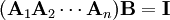
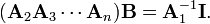
$(\mathbf{A}_1\mathbf{A}_2\cdots \mathbf{A}_n)\mathbf{B}=\mathbf{I}$

where B is the inverse matrix of the product. To remove A₁ from the product, we can then write

$\mathbf{A}_1^{-1}(\mathbf{A}_1\mathbf{A}_2\cdots \mathbf{A}_n)\mathbf{B}=\mathbf{A}_1^{-1}\mathbf{I}$

which would reduce the equation to

$(\mathbf{A}_2\mathbf{A}_3\cdots \mathbf{A}_n)\mathbf{B}=\mathbf{A}_1^{-1}\mathbf{I}.$

Likewise, then, from

$\mathbf{A}_2^{-1}(\mathbf{A}_2\mathbf{A}_3\cdots \mathbf{A}_n)\mathbf{B}=\mathbf{A}_2^{-1}\mathbf{A}_1^{-1}\mathbf{I}$

which simplifies to

$(\mathbf{A}_3\mathbf{A}_4\cdots \mathbf{A}_n)\mathbf{B}=\mathbf{A}_2^{-1}\mathbf{A}_1^{-1}\mathbf{I}.$

If one repeat the process up to A_n, the equation becomes

$\mathbf{B}=\mathbf{A}_n^{-1}\mathbf{A}_{n-1}^{-1}\cdots \mathbf{A}_2^{-1}\mathbf{A}_1^{-1}\mathbf{I}$

$\mathbf{B}=\mathbf{A}_n^{-1}\mathbf{A}_{n-1}^{-1}\cdots \mathbf{A}_2^{-1}\mathbf{A}_1^{-1}$

but B is the inverse matrix, i.e. $\mathbf{B} = (\mathbf{A}_1\mathbf{A}_2\cdots \mathbf{A}_n)^{-1}$ so the property is established.

[edit] Density of invertible matrices

Over the field of real numbers, the set of singular n-by-n matrices, considered as a subset of $R^{n \times n}$ , is a null set, i.e., has Lebesgue measure zero. This is true because singular matrices are the roots of the polynomial function in the entries of the matrix given by the determinant. Thus in the language of measure theory, almost all n-by-n matrices are invertible. Intuitively, this means that if you pick a random square matrix over the reals, the probability that it will be singular is zero; n randomly picked vectors will form a basis for a n-space with probability 1.

Furthermore the n-by-n invertible matrices are a dense open set in the topological space of all n-by-n matrices. Equivalently, the set of singular matrices is closed and nowhere dense in the space of n-by-n matrices.

In practice however, one may encounter non-invertible matrices. And in numerical calculations, matrices which are invertible, but close to a non-invertible matrix, can still be problematic; such matrices are said to be ill-conditioned.

[edit] Methods of matrix inversion

[edit] Gaussian elimination

Gauss–Jordan elimination is an algorithm that can be used to determine whether a given matrix is invertible and to find the inverse. An alternative is the LU decomposition which generates an upper and a lower triangular matrices which are easier to invert. For special purposes, it may be convenient to invert matrices by treating mn-by-mn matrices as m-by-m matrices of n-by-n matrices, and applying one or another formula recursively (other sized matrices can be padded out with dummy rows and columns). For other purposes, a variant of Newton's method may be convenient (particularly when dealing with families of related matrices, so inverses of earlier matrices can be used to seed generating inverses of later matrices).

[edit] Analytic solution

Main article: Cramer's rule

Writing another special matrix of cofactors, known as an adjugate matrix, can also be an efficient way to calculate the inverse of small matrices, but this recursive method is inefficient for large matrices. To determine the inverse, we calculate a matrix of cofactors:

$\mathbf{A}^{-1}={1 \over \begin{vmatrix}\mathbf{A}\end{vmatrix}}\left(\mathbf{C}_{ij}\right)^{\mathrm{T}}={1 \over \begin{vmatrix}\mathbf{A}\end{vmatrix}}\left(\mathbf{C}_{ji}\right)={1 \over \begin{vmatrix}\mathbf{A}\end{vmatrix}} \begin{pmatrix} \mathbf{C}_{11} & \mathbf{C}_{21} & \cdots & \mathbf{C}_{n1} \\ \mathbf{C}_{12} & \mathbf{C}_{22} & \cdots & \mathbf{C}_{n2} \\ \vdots & \vdots & \ddots & \vdots \\ \mathbf{C}_{1n} & \mathbf{C}_{2n} & \cdots & \mathbf{C}_{nn} \\ \end{pmatrix}$

where |A| is the determinant of A, C_ij is the matrix cofactor, and A^T represents the matrix transpose.

For most practical applications, it is not necessary to invert a matrix to solve a system of linear equations; however, for a unique solution, it is necessary that the matrix involved be invertible.

Decomposition techniques like LU decomposition are much faster than inversion, and various fast algorithms for special classes of linear systems have also been developed.

[edit] Inversion of 2×2 matrices

The cofactor equation listed above yields the following result for 2×2 matrices. Inversion of these matrices can be done easily as follows: ^[2]

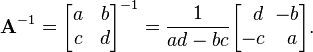
$\mathbf{A}^{-1} = \begin{bmatrix} a & b \\ c & d \\ \end{bmatrix}^{-1} = \frac{1}{ad - bc} \begin{bmatrix} \,\,\,d & \!\!-b \\ -c & \,a \\ \end{bmatrix}.$

This is possible because 1/(ad-bc) is the reciprocal of the determinant of the matrix in question, and the same strategy could be used for other matrix sizes.

[edit] Blockwise inversion

Matrices can also be inverted blockwise by using the following analytic inversion formula:

$\begin{bmatrix} \mathbf{A} & \mathbf{B} \\ \mathbf{C} & \mathbf{D} \end{bmatrix}^{-1} = \begin{bmatrix} \mathbf{A}^{-1}+\mathbf{A}^{-1}\mathbf{B}(\mathbf{D}-\mathbf{CA}^{-1}\mathbf{B})^{-1}\mathbf{CA}^{-1} & -\mathbf{A}^{-1}\mathbf{B}(\mathbf{D}-\mathbf{CA}^{-1}\mathbf{B})^{-1} \\ -(\mathbf{D}-\mathbf{CA}^{-1}\mathbf{B})^{-1}\mathbf{CA}^{-1} & (\mathbf{D}-\mathbf{CA}^{-1}\mathbf{B})^{-1} \end{bmatrix}$

$(1)\,$

where A, B, C and D are matrix sub-blocks of arbitrary size. (A and D must, of course, be square, so that they can be inverted). This strategy is particularly advantageous if A is diagonal and D−CA⁻¹B (the Schur complement of A) is a small matrix, since they are the only matrices requiring inversion. This technique was reinvented several times and is due to Hans Bolz (1923), who used it for the inversion of geodetic matrices, and Tadeusz Banachiewicz (1937), who generalized it and proved its correctness.

The nullity theorem says that the nullity of A equals the nullity of the sub-block in the lower right of the inverse matrix, and that the nullity of B equals the nullity of the sub-block in the upper right of the inverse matrix.

The inversion procedure that led to Equation (1) performed matrix block operations that operated on C and D first. Instead, if A and B are operated on first, the result is

$\begin{bmatrix} \mathbf{A} & \mathbf{B} \\ \mathbf{C} & \mathbf{D} \end{bmatrix}^{-1} = \begin{bmatrix} (\mathbf{A}-\mathbf{BD}^{-1}\mathbf{C})^{-1} & -(\mathbf{A}-\mathbf{BD}^{-1}\mathbf{C})^{-1}\mathbf{BD}^{-1} \\ -\mathbf{D}^{-1}\mathbf{C}(\mathbf{A}-\mathbf{BD}^{-1}\mathbf{C})^{-1} & \mathbf{D}^{-1}+\mathbf{D}^{-1}\mathbf{C}(\mathbf{A}-\mathbf{BD}^{-1}\mathbf{C})^{-1}\mathbf{BD}^{-1}\end{bmatrix}$

$(2)\,$

Equating Equations (1) and (2) leads to

$(\mathbf{A}-\mathbf{BD}^{-1}\mathbf{C})^{-1} = \mathbf{A}^{-1}+\mathbf{A}^{-1}\mathbf{B}(\mathbf{D}-\mathbf{CA}^{-1}\mathbf{B})^{-1}\mathbf{CA}^{-1}\,$

$(3)\,$

$(\mathbf{A}-\mathbf{BD}^{-1}\mathbf{C})^{-1}\mathbf{BD}^{-1} = \mathbf{A}^{-1}\mathbf{B}(\mathbf{D}-\mathbf{CA}^{-1}\mathbf{B})^{-1}\,$

$\mathbf{D}^{-1}\mathbf{C}(\mathbf{A}-\mathbf{BD}^{-1}\mathbf{C})^{-1} = (\mathbf{D}-\mathbf{CA}^{-1}\mathbf{B})^{-1}\mathbf{CA}^{-1}\,$

$\mathbf{D}^{-1}+\mathbf{D}^{-1}\mathbf{C}(\mathbf{A}-\mathbf{BD}^{-1}\mathbf{C})^{-1}\mathbf{BD}^{-1} = (\mathbf{D}-\mathbf{CA}^{-1}\mathbf{B})^{-1}\,$

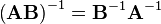
where Equation (3) is the matrix inversion lemma, which is equivalent to the binomial inverse theorem.

[edit] The derivative of the matrix inverse

Suppose that the matrix A depends on a parameter t. Then the derivative of the inverse of A with respect to t is given by

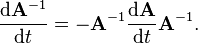
$\frac{\mathrm{d}\mathbf{A}^{-1}}{\mathrm{d}t} = - \mathbf{A}^{-1} \frac{\mathrm{d}\mathbf{A}}{\mathrm{d}t} \mathbf{A}^{-1}.$

This formula can be found by differentiating the identity

$\mathbf{A}^{-1}\mathbf{A} = \mathbf{I}.\,$

[edit] The Moore-Penrose pseudoinverse

Some of the properties of inverse matrices are shared by (Moore-Penrose) pseudoinverses, which can be defined for any m-by-n matrix.

[edit] Matrix inverses in real-time simulations

Matrix inversion plays a significant role in computer graphics, particularly in 3D graphics rendering and 3D simulations. Examples include screen-to-world ray casting, world-to-subspace-to-world object transformations, and physical simulations. The problem is usually the numerical complexity of calculating the inverses of 3×3 and 4×4 matrices. Compared to matrix multiplication or creation of rotation matrices, matrix inversion is several orders of magnitude slower. There are existing solutions which use hand-crafted assembly language routines and SIMD processor extensions (SSE, SSE2, Altivec) that address this problem and which achieve a performance improvement of as much as five times.

[edit] See also

[edit] Notes

^ Horn, Roger A.; Johnson, Charles R. (1985), Matrix Analysis, Cambridge University Press, p. 14, ISBN 978-0-521-38632-6 .
^ Strang, Gilbert (2006). Linear Algebra and Its Applications. Thomson Brooks/Cole. pp. 46. ISBN 0-03-010567-6.

[edit] References

Cormen, Thomas H.; Leiserson, Charles E., Rivest, Ronald L., Stein, Clifford (2001) [1990]. "28.4: Inverting matrices". Introduction to Algorithms (2nd ed.). MIT Press and McGraw-Hill. pp. pp. 755–760. ISBN 0-262-03293-7.

[edit] External links

MIT Linear Algebra Lecture on Inverse Matrices
LAPACK is a collection of FORTRAN subroutines for solving dense linear algebra problems
ALGLIB includes a partial port of the LAPACK to C++, C#, Delphi, etc.
Online Inverse Matrix Calculator using AJAX
Inverse Matrix Calculator
Moore Penrose Pseudoinverse
Inverse of a Matrix Notes
Module for the Matrix Inverse
Calculator for Singular or Non-Square Matrix Inverse
Derivative of inverse matrix on PlanetMath

[0] Horn, Roger A.; Johnson, Charles R. (1985), Matrix Analysis, Cambridge University Press, p. 14, ISBN 978-0-521-38632-6 .

[1] Strang, Gilbert (2006). Linear Algebra and Its Applications. Thomson Brooks/Cole. pp. 46. ISBN 0-03-010567-6.

[1]

[2]

Invertible matrix

From Wikipedia, the free encyclopedia

Contents

[edit] Properties of invertible matrices

[edit] Proof for matrix product rule

[edit] Density of invertible matrices

[edit] Methods of matrix inversion

[edit] Gaussian elimination

[edit] Analytic solution

[edit] Inversion of 2×2 matrices

[edit] Blockwise inversion

[edit] The derivative of the matrix inverse

[edit] The Moore-Penrose pseudoinverse

[edit] Matrix inverses in real-time simulations

[edit] See also

[edit] Notes

[edit] References

[edit] External links

Views

Personal tools

Navigation

Search

Interaction

Toolbox

Languages